Spreadsheet: Functions and Charts

Choose the correct option

Question 1

In what way a cell is addressed in a worksheet?

1. Using column name followed by row number.
2. Using row number followed by column name.
3. By scrolling up and down.
4. By calculating the distance from reference cell.

Answer

Using column name followed by row number.

Reason — The address of a cell consists of the column letter followed by the row number.

Question 2

In which position, the sheet tab is located on the screen?

1. At the top left corner
2. At the top right corner
3. At the bottom right corner
4. At the bottom left corner

Answer

At the bottom left corner

Reason — The sheet tab is located at the bottom left corner on the screen.

Question 3

In what way a worksheet can be erased?

1. By right clicking the sheet name and selecting 'delete' option from the drop-down list.
2. By right clicking the sheet name and selecting 'erase' option from the drop-down list.
3. By right clicking the sheet name and selecting 'remove' option from the drop-down list.
4. None of the above.

Answer

By right clicking the sheet name and selecting 'delete' option from the drop-down list.

Reason — A worksheet can be erased by right clicking the sheet name and selecting 'delete' option from the drop-down list.

Question 4

Which of the following functions is used to add the values of consecutive cells?

1. total( )
2. sum( )
3. add( )
4. None of the above

Answer

sum( )

Reason — sum( ) function calculates the sum of all the values of the specified cells.

Question 5

The max( ) function is used to find the maximum of:

1. two values
2. three values
3. any number of values
4. none of them

Answer

Any number of values

Reason — Max( ) function returns the highest value among all the values of the specified cells or the range of cells.

Question 6

Count( ) function is used to find the

1. number of elements in a range of cells.
2. frequency of an element in a range of cells.
3. number of elements starting with a specific digit.
4. number of elements ending with a specific digit.

Answer

Number of elements in a range of cells

Reason — The count function enables a user to count the number of cells in a range that contain numbers.

Question 7

Which of the following is not a pictorial representation of data?

1. Chart
2. Graph
3. SmartArt
4. Range of cells

Answer

Range of cells

Reason — A range of cells is a group of cells that has been selected.

Question 8

What is meant by customising a chart?

1. Sending a chart to the customer
2. Modifying a chart as per requirement
3. Receiving a chart through e-mail
4. Declaring a chart title

Answer

Modifying a chart as per requirement

Reason — Customising a chart means modifying a chart as per requirement.

State True or False

Question 1

A range of cells is a group of cells that has been selected.
True

Question 2

A spreadsheet can contain only numeric data.
False

Question 3

You can insert a chart but not a clipart in a worksheet.
False

Question 4

The cell in which the cell pointer is located in a worksheet, is referred to as the active cell.
True

Question 5

You can select a range of data as per your choice in a spreadsheet.
True

Fill in the blanks

Question 1

Charts are the pictorial representation of data values stored in the worksheet.

Question 2

When the corresponding cell address changes with reference to a new cell address, it is known as relative reference.

Question 3

By default, MS Excel provides three worksheets in a workbook.

Question 4

The built-in formulae for specific numeric/non-numeric processing are called functions.

Question 5

A range of cells is a rectangular block consisting of a few cells, an entire row, an entire column or the whole worksheet.

Write the format of the functions used in MS Excel to perform the following tasks

Question 1

To calculate the average of 82, 67, 80, 74 and 95.

Answer

=AVERAGE(82,67,80,74,95)

Question 2

To find the highest value of the cell references from D3 to K3.

Answer

=MAX(D3:K3)

Question 3

To calculate the sum of the first five multiples of 7.

Answer

=SUM(7,14,21,28,35)

Question 4

To determine the lowest value of the cell references from A4 to A12.

Answer

=MIN(A4:A12)

Question 5

To find the sum of all the prime numbers from 1 to 10.

Answer

=SUM(2,3,5,7)

Question 6

To find the arithmetical mean of the cell references from E4 to K4.

Answer

=AVERAGE(E4:K4)

Spot the error in each of the following

Question 1

=SUM ('C9':C14)

Answer

=SUM(C9:C14)

Question 2

=$B*$3*C$

Answer

=$B$3 * C$4

Question 3

=COUNT(9, 12, 17, 26, A$)

Answer

=COUNT(9, 12, 17, 26)

This will give the output as 4 since there are 4 numeric values given as input to the count function.

Question 4

=AVERAGE(A1:An)/n

Answer

=AVERAGE(A1:An)

where 'n' is the row number of the cell till where the average is required.

Question 5

=MAX('19', 70, 101)

Answer

=MAX(19,70,101)

Question 5

=ADD(24+54+77-38)

Answer

=SUM(24,54,77)-38

Case-Study Based Questions

Question 1

Given below is a table containing 'Rate/gm' and 'Wt in gm' in columns A and B respectively. Cell D1 contains GST as 5% (i.e. 0.05). The cost (including GST) of each item is to be calculated and stored in the corresponding cells of column C as (Rate/gm) * Wt in gm * GST.

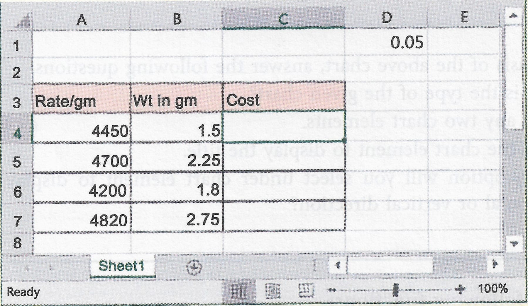
Based on the above case, answer the following questions:

(a) Which of the following represents cell D1 as absolute?

1. $D1$
2. D$1$
3. $D$1
4. D1$

(b) What will happen when cell C1 is absolute and used in the formula to find cost in the cells from C4 to C7?

1. All cell values from C4 to C7 will become 0 (zero).
2. The cell value D1 will be shifted into the cell C1.
3. The cell value D1 will be copied into the cell C1.
4. All the cell values from C4 to C7 will occupy same non-zero values.

(c) What will be the formula to calculate the cost in column C4?

1. A4 * B4 * D1
2. A4 * B4 * $D$1
3. A4 * $B4$ * D1
4. $A4$ * $B4$ * $d4$

(d) What will be the formula to calculate the cost in column C7?

1. $A$7 * B7 * D1
2. A7 * B7 * $D$1
3. A$7$ * B$7$ * D1
4. A7 * B7 * $D1$

Answer

(a) $D$1

Reason — We add '$' sign before a column and row to make it absolute.

(b) All cell values from C4 to C7 will become 0 (zero).

Reason — The result is zero because cell C1 is empty and as a result its numeric value will be taken as 0.

(c) A4 * B4 * $D$1.

Reason — We add '$' sign before a column and row to make it absolute. Hence the value of GST % in cell D1 remains the same while the cost changes according to cell C4, C5...and so on.

Note — There is a misprint in the options. Cell D1 has been incorrectly referred to as C1. This error has been fixed in the question here.

(d) A7 * B7 * $D$1

Reason — A7 and B7, being relative references will change while $D$1 being absolute reference will remain the same.

Question 2

Given below is a chart which shows the comparative study of the prices of TV sets of various companies:

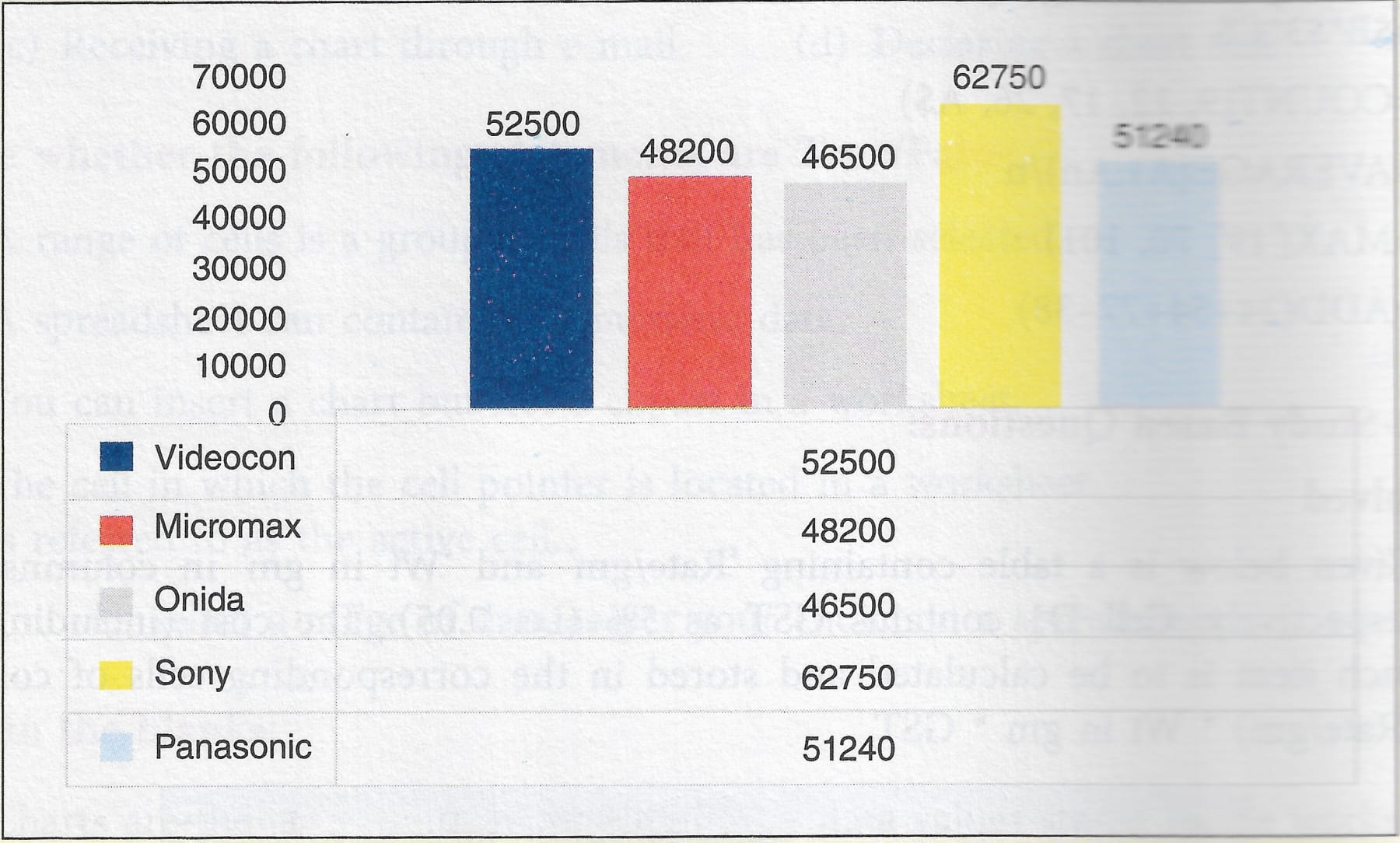
On the basis of the above chart, answer the following questions:

(a) What is the type of the given chart?

(b) Name any two chart elements.

(c) Name the chart element to display the title.

(d) Which option will you select under chart element to display information along horizontal or vertical direction?

Answer

(a) The given chart is a 2D column chart.

(b) Two chart elements are Chart Title and Axis Title.

(c) Chart Title displays the title of the chart.

(d) One will select Axis Title to display information along horizontal or vertical direction.

Explain the following functions

Question 1

=SUM(C5:H5)

Answer

This function calculates the sum of the cell references from C5 to H5.

Question 2

=AVERAGE (K12:K50)

Answer

This function calculates the average of the cell references from K12 to K50.

Question 3

=COUNT (B15:B35)

Answer

This function counts the number of cells which contain numeric values, in the range of cells from B15 to B35.

Question 4

=MAX (A4:A14)

Answer

This function finds the highest value among the cell references from A4 to A14.

Explain the three types of referencing

Question 1

Relative Referencing

Answer

In Relative Referencing, when the formula is copied to a new cell, the corresponding cell address changes with reference to the new cell address.

For example, consider the formula '=SUM(A1:A5)' in A6 for calculating the total from A1 to A5. Here the relative positions of the cells are specified. When this formula is copied to B6 or C6, it will automatically get adjusted as below:

For B6, it will become =SUM(B1:B5)
For C6, it will become =SUM(C1:C5)

Question 2

Absolute Referencing

Answer

In Absolute Referencing, the address of the cells is specified in a way that it remains constant when the formula is copied to a new cell. To keep the cell value absolute, apply the '$' sign before the column name, as well as the row number.

For example, let us consider that cell C6 has the formula =A6*B6*$F$3. The formula takes the relative cell values from A6 and B6, and the absolute value from the cell F3. When this formula is copied to C7 or C8, it will automatically get adjusted as below:

For C7, it will become =A7*B7*$F$3
For C8, it will become =A8*B8*$F$3

Notice that the relative reference changes but the absolute reference $F$3 remains the same.

Question 3

Mixed Referencing

Answer

Mixed Referencing is a combination of relative and absolute referencing. In this reference, the data of one cell is kept absolute and other is made relative and finally they are operated together in a formula.

For example, let us consider that cell B5 has the formula =$B$3*B$4. When this formula is copied to C5 and D5, it will automatically get adjusted as below:

For C5, it will become =$B$3*C$4
For D5, it will become =$B$3*D$4

Define the functions

Question 1

SUM ( )

Answer

This function calculates the total of all the values of the specified cells and returns the result to the cell where the cell pointer is located.

Its syntax is:
=SUM(number1, number2, .......) where argument type is Number and return type is Number.

To find the sum of the cell values ranging from A1, A2, A3, ........ to An, the function will be written as:
=SUM(A1, A2, A3, ......., An)
      OR
=SUM(A1:An)

Question 2

AVERAGE ( )

Answer

This function takes all the values of the specified cells and returns the average of the cell values in the active cell.

Its syntax is:
=AVERAGE(number1, number2, .......) where argument type is Number and return type is Number.

To find the average of the cell values ranging from A1, A2, A3, ........ to An, the function will be written as:
=AVERAGE(A1, A2, A3, ......., An)
      OR
=AVERAGE(A1:An)

Question 3

MAX ( )

Answer

This function returns the highest value among all the values of the specified cells or the range of cells.

Its syntax is:
=MAX(number1, number2, .......) where argument type is Number and return type is Number.

To know the highest of the cell values ranging from A1, A2, A3, ........ to An, the function will be written as:
=MAX(A1, A2, A3, ......., An)
      OR
=MAX(A1:An)

Question 4

MIN ( )

Answer

This function returns the lowest value among the values of the specified cells or the range of cells.

Its syntax is:
=MIN(number1, number2, .......) where argument type is Number and return type is Number.

To know the lowest of the cell values ranging from A1, A2, A3, ........ to An, the function will be written as:
=MIN(A1, A2, A3, ......., An)
      OR
=MIN(A1:An)

Short Answer Questions

Question 1

What are the points to be taken care of while writing the format of a function in MS Excel?

Answer

The following points must be taken care of while writing the format of a function in MS Excel:

1. Each function must begin with an 'equal to' (=) sign.
2. Parenthesis is used to indicate the opening and closing of a function.
3. Arguments are written within the parenthesis.
4. Commas are used to separate the arguments.

Question 2

What is meant by cell reference?

Answer

Every cell in a worksheet has a cell address, by which it is referred and when this address is used in a formula, it is known as cell referencing.

MS Excel provides three different ways to refer to a cell-

1. Relative Referencing
2. Absolute Referencing
3. Mixed Referencing

Question 3

Define Sheet Tab.

Answer

In MS Excel, the tab which displays various worksheets in a workbook is called the 'Sheet Tab'. It is located at the bottom left corner of the excel window. By default, the system displays only one sheet named Sheet1.

Question 4

Explain the term 'Range of Cells' in a spreadsheet.

Answer

When more than one cells are selected in a worksheet, the selected cells are known as range of cells. A range is specified by giving the addresses of the first cell and the last cell to be included in the range.

Question 5

What do you understand by chart? Explain with reference to MS Excel.

Answer

A chart is a pictorial representation of data used to communicate information in a better way. It helps in better visualisation, comparison and relationship between data.

MS Excel provides different types of charts such as column chart, line chart, pie chart, bar chart, etc. from which the user can select as per his/her need.

Write all the steps to perform the following tasks in MS Excel

Question 1

Naming a Worksheet

Answer

To name a worksheet, follow these steps:

Step 1 — Double-click the name of the worksheet on the sheet tab.

Step 2 — Enter the name and press 'Enter' key.

Question 2

Renaming a Worksheet

Answer

To rename a worksheet, follow these steps:

Step 1 — Double-click the name of the worksheet on the sheet tab.

Step 2 — Enter the new name and press 'Enter' key.

Question 3

Deleting a worksheet

Answer

To delete a worksheet, follow these steps:

Step 1 — Right-click on the sheet name on the Sheet Tab that you want to delete.

Step 2 — Select the 'Delete' option from the pop-up list.

Question 4

Selecting a partial range in a row

Answer

To select a partial range in a row, follow these steps:

Step 1 — Select the first cell.

Step 2 — Keeping the left mouse button pressed, drag the mouse to select the desired number of cells in a row.

Step 3 — Release the mouse button.

Question 5

Selecting multiple columns in a worksheet

Answer

To select multiple columns in a worksheet, follow these steps:

Step 1 — Select or bring the mouse pointer to the column header of a column from where consecutive columns are to be selected.

Step 2 — Press the left mouse button to select required number of consecutive columns.

Step 3 — Release the mouse button.

Question 6

Preparing a chart by using a sample data table

Answer

To prepare a chart by using a sample data table, follow these steps:

Step 1 — Select the range of cells whose data is to be represented.

Step 2 — Click the 'Insert' tab on the ribbon.

Step 3 — Click and select the type of chart (say, Column chart) from the 'Charts' group. A drop-down list opens.

Step 4 — Select the desired chart (say, a 2-D Column). The data will be displayed in the form of the chart selected.

MS Excel Task

You have purchased some textbooks from a bookstore, as given below:

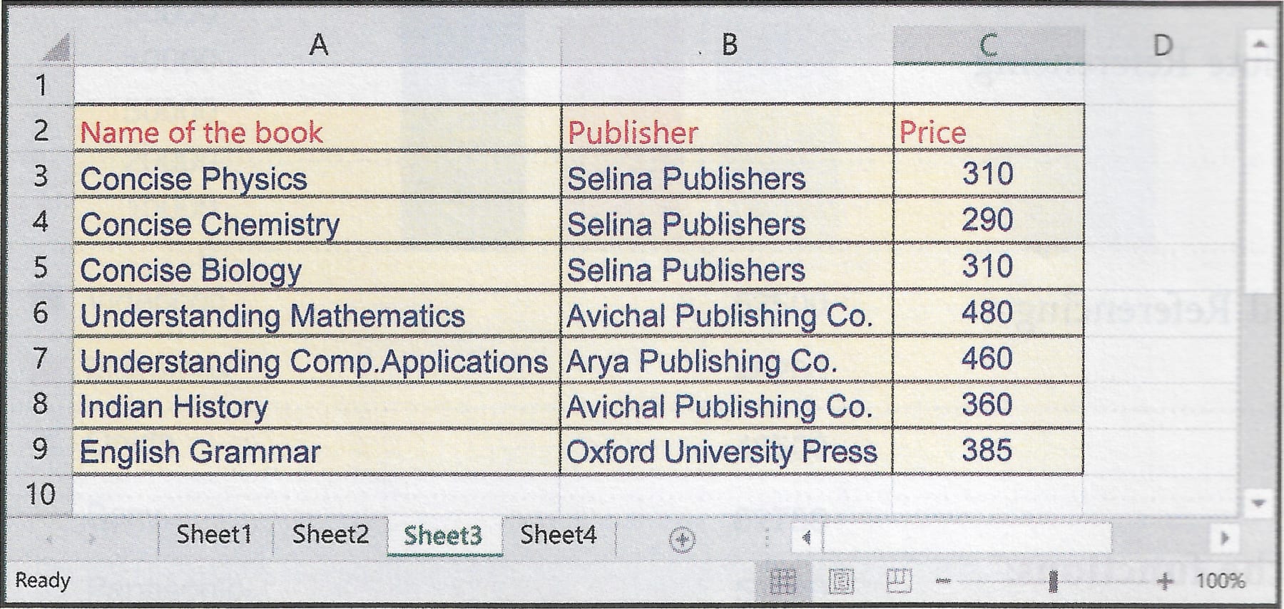
Write the steps involved to perform the following tasks in MS Excel on the table given above.

Question 1

Find the average price of the books.

Answer

To find the average price of the books, follow these steps:

Step 1 — Select the cell where you want to display the average price of the books.

Step 2 — Type the formula =AVERAGE(C3:C9) in the cell.

Step 3 — Press 'Enter' key.

The average price of the books will be calculated.

Question 2

If the bookseller offers 10% discount, then calculate the amount to be paid to the shopkeeper.

Answer

To calculate the amount to be paid to the shopkeeper, follow these steps:

Step 1 — Select cell D3.

Step 2 — Write the formula =C3-(C3*0.1) and press enter key.

Step 3 — Select cell D3 again and drag the cell handle from D3 till D9.

Step 4 — Select cell D10.

Step 5 — Write the formula =SUM(D3:D9) and press enter key.

Cell D10 shows the amount payable to the shopkeeper.

Question 3

Find the price of the book which had the highest price among the books you bought.

Answer

To find the price of the book which had the highest price among the books you bought, follow these steps:

Step 1 — Select the cell where you want to display the result.

Step 2 — Type the formula =MAX(C3:C9) in the cell.

Step 3 — Press 'Enter' key.

The price of the most expensive book will be displayed.

Question 4

Calculate the total amount paid at the bookstore.

Answer

To calculate the total amount to be paid to the shopkeeper, follow these steps:

Step 1 — Select the cell C10.

Step 2 — Type the formula =SUM(C3:C9) in the cell.

Step 3 — Press 'Enter' key.

C10 will display the total amount to be paid to the shopkeeper.