
Which of the following are statistical questions?
(a) What is the price of a tennis ball in India?
(b) How old are the dogs that live on this street?
(c) What fraction of the students in your class like walking up a hill?
(d) Do you like reading?
(e) Approximately how many bricks are in this wall?
(f) Who was the best bowler in the match yesterday?
(g) What was the rainfall pattern in Barmer last year?
Answer
A statistical question is a question that can be answered by collecting data. Such a question expects the answers to vary, so the data has to be collected, organised and analysed before a conclusion is drawn.
(a) The price of a tennis ball is not the same everywhere — it varies from shop to shop, from brand to brand and from place to place. To answer this, prices have to be collected from many places and analysed.
Hence, it is a statistical question.
(b) The dogs living on a street are of different ages. To answer this, the ages of all the dogs on the street have to be collected and analysed.
Hence, it is a statistical question.
(c) Different students in the class have different likings. To answer this, every student in the class has to be asked and then the required fraction has to be calculated.
Hence, it is a statistical question.
(d) This question is put to one person and is answered by a simple 'yes' or 'no'. No data has to be collected or analysed to answer it.
Hence, it is not a statistical question.
(e) A particular wall has a fixed number of bricks. The answer is a single number, obtained by counting (or by estimating from the size of the wall and of a brick). The answer does not vary.
Hence, it is not a statistical question.
(f) In a particular match, the bowling figures of yesterday's match are already fixed. The answer is a single fact that can be read directly from the scorecard of that one match.
Hence, it is not a statistical question.
(g) The rainfall in Barmer changes from day to day and from month to month. To describe the pattern of last year, the rainfall data of the whole year has to be collected and analysed.
Hence, it is a statistical question.
∴ (a), (b), (c) and (g) are statistical questions, while (d), (e) and (f) are not.
The runs scored by Shubman and Yashasvi in a cricket series are given in the table below. Who do you think performed better?
| Match 1 | Match 2 | Match 3 | Match 4 | |
|---|---|---|---|---|
| Shubman | 0 | 17 | 21 | 90 |
| Yashasvi | 67 | 55 | 18 | 35 |
Answer
Both the players have played 4 matches each, so their performances can be compared using the total runs, the average runs and the spread of the runs.
Total runs scored by Shubman = 0 + 17 + 21 + 90 = 128 runs
Total runs scored by Yashasvi = 67 + 55 + 18 + 35 = 175 runs
Total number of matches = 4
Average runs scored by Shubman =
Average runs scored by Yashasvi =
Comparing the two players:
(i) Yashasvi's total (175 runs) is more than Shubman's total (128 runs).
(ii) Yashasvi's average (43.75 runs) is more than Shubman's average (32 runs).
(iii) Range of Shubman's scores = 90 - 0 = 90 runs, and range of Yashasvi's scores = 67 - 18 = 49 runs. So Yashasvi's batting is more consistent.
Shubman does have the highest individual score of the series (90 runs), but in every other measure Yashasvi is ahead.
Hence, Yashasvi performed better in this series.
The table below shows the runs scored by these two players in another series. Who do you think performed better in this series?
| Match 1 | Match 2 | Match 3 | Match 4 | Match 5 | |
|---|---|---|---|---|---|
| Shubman | 23 | 07 | 10 | 52 | 18 |
| Yashasvi | 26 | 53 | 02 | - | 15 |
(i) What do you think of Vaishnavi's statement?
(ii) Can a single number act as a representative of a group of numbers? For example, can we represent Shubman's or Yashasvi's batting in this series with one number? Discuss.
Answer
The dash '-' in Match 4 means that Yashasvi did not play that match. So Shubman played 5 matches while Yashasvi played only 4 matches.
Since the number of matches played is different, the totals cannot be compared directly. The averages must be compared.
Total runs scored by Shubman = 23 + 7 + 10 + 52 + 18 = 110
Total number of matches = 5
Average runs scored by Shubman =
Total runs scored by Yashasvi = 26 + 53 + 2 + 15 = 96
Total number of matches = 4
Average runs scored by Yashasvi =
As 24 > 22, Yashasvi's average number of runs per match is higher than Shubman's.
Hence, Yashasvi performed better in this series.
(i)
Vaishnavi's statement is — 'Here, Shubman performed better since his total is 110 runs, while Yashasvi's total is 96 runs.'
This comparison is not correct, because Shubman played 5 matches while Yashasvi played only 4 matches.
When two groups have different numbers of values, comparing only their totals may not give a fair comparison. In such cases, the average (Arithmetic Mean) is a better representative value.
Average runs per match of Shubman = 110 ÷ 5 = 22 runs
Average runs per match of Yashasvi = 96 ÷ 4 = 24 runs
Since 24 > 22, Yashasvi performed better on average.
Hence, Vaishnavi's statement is not correct.
(ii)
Yes, a single number can act as a representative of a group of numbers.
A representative number can be obtained by adding all the values in the group and dividing the total by the number of values. This number is called the average or Arithmetic Mean.
Average or Arithmetic Mean =
For this series:
Average runs scored by Shubman = runs
Average runs scored by Yashasvi = runs
The average represents the batting performance of each player with a single number and allows a fair comparison, even though they played a different number of matches.
Hence, the average (Arithmetic Mean) can be used as a representative value for a group of numbers.
Shreyas is playing with a bat and a ball — but not cricket. He counts the number of times he can bounce the ball on the bat before it falls to the ground. The data for 8 attempts is 6, 2, 9, 5, 4, 6, 3, 5. Calculate the average number of bounces of the ball that Shreyas is able to make with his bat.
Answer
Number of attempts = 8
Sum of all the values in the data = 6 + 2 + 9 + 5 + 4 + 6 + 3 + 5 = 40
Number of values in the data = 8
Average number of bounces =
Hence, Shreyas is able to make 5 bounces on average with his bat.
Two friends are training to run a 100 m race. Their running times over the past week are given in seconds — Nikhil: 17, 18, 17, 16, 19, 17, 18; Sunil: 20, 18, 18, 17, 16, 16, 17. Who on average ran quicker?
Answer
Total running time of Nikhil = 17 + 18 + 17 + 16 + 19 + 17 + 18 = 122 seconds
Total running time of Sunil = 20 + 18 + 18 + 17 + 16 + 16 + 17 = 122 seconds
Number of observations = 7
Nikhil's average time =
Sunil's average time =
Since both Nikhil and Sunil have the same average running time of 17.43 seconds (approx.), both of them ran equally quick on average.
Hence, neither Nikhil nor Sunil ran quicker than the other on average.
The enrolment in a school during six consecutive years was as follows: 1555, 1670, 1750, 2013, 2040, 2126. Find the mean enrolment in the school during this period.
Answer
Sum of all observations = 1555 + 1670 + 1750 + 2013 + 2040 + 2126 = 11154
Number of observations = 6
Mean enrolment =
Hence, the mean enrolment in the school during this period is 1859.
The table shows the monthly price of onions, in rupees per kilogram (kg), at two towns. Where are onions costlier, according to you?
| Month | Yahapur | Wahapur |
|---|---|---|
| January | 25 | 19 |
| February | 24 | 17 |
| March | 26 | 23 |
| April | 28 | 30 |
| May | 30 | 38 |
| June | 35 | 35 |
| July | 39 | 42 |
| August | 43 | 39 |
| September | 49 | 53 |
| October | 56 | 60 |
| November | 59 | 52 |
| December | 44 | 42 |
Answer
Let us compare the two towns in a few different ways:
1. Total of the prices
Total price at Yahapur = ₹ (25 + 24 + 26 + 28 + 30 + 35 + 39 + 43 + 49 + 56 + 59 + 44) = ₹458
Total price at Wahapur = ₹ (19 + 17 + 23 + 30 + 38 + 35 + 42 + 39 + 53 + 60 + 52 + 42) = ₹450
Since ₹ 458 > ₹ 450, the total is higher for Yahapur.
2. Month-wise comparison
- Yahapur has higher prices in 6 months.
- Wahapur has higher prices in 5 months.
- The prices are the same in 1 month (June).
3. Highest and lowest prices
Highest price at Yahapur = ₹59 and highest price at Wahapur = ₹60.
Lowest price at Yahapur = ₹24 and lowest price at Wahapur = ₹17.
Thus, Wahapur has both the highest and the lowest monthly prices, showing that its prices vary more.
Judging by the total (and hence the average) price over the whole year, and by the number of months in which the price is higher, onions are costlier at Yahapur — though only by a small margin.
Hence, taking the whole year into account, onions are slightly costlier at Yahapur.
In the following figure, each dot represents the monthly price of onions.
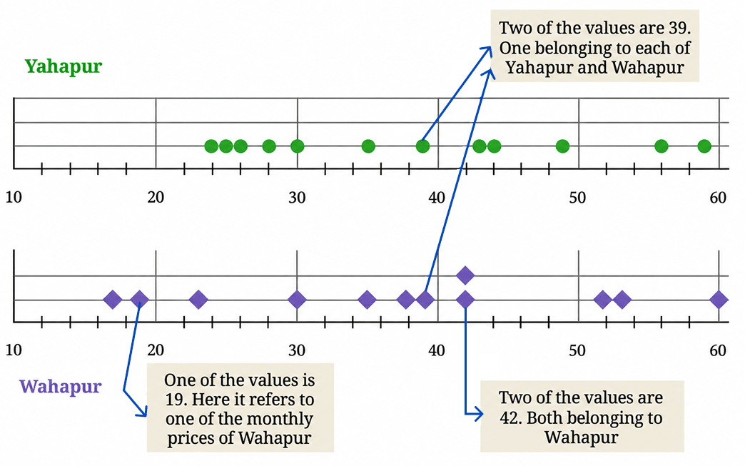
(i) Does this visualisation capture all the data presented in the tables earlier?
(ii) Looking at it, can we tell the price of onions in Yahapur in the month of January?
(iii) Find the average price of onions at Yahapur and Wahapur.
(iv) What else do you wonder about?
Answer
(i)
Each dot in the dot plot represents one monthly price. There are 12 dots for Yahapur and 12 dots for Wahapur, so all the monthly price values are shown.
However, the dot plot arranges the prices according to their values. It does not show which month a particular price belongs to.
Hence, the dot plot captures all the price values, but not the month to which each price belongs.
(ii)
No, we cannot tell the price of onions in Yahapur in the month of January by looking at these plots.
The dot plot sorts the prices in increasing order along the horizontal line, so the original month-wise sequence of the values is lost. Looking at a dot on the Yahapur line, we can only say that some month had that price; we cannot say which month it was.
Hence, we cannot tell from the dot plot the price of onions in Yahapur in the month of January.
(iii)
Total price of onions at Yahapur = 25 + 24 + 26 + 28 + 30 + 35 + 39 + 43 + 49 + 56 + 59 + 44 = 458
Number of all observations = 12
Average price at Yahapur =
Total price of onions at Wahapur = 19 + 17 + 23 + 30 + 38 + 35 + 42 + 39 + 53 + 60 + 52 + 42 = 450
Number of all observations = 12
Average price at Wahapur =
Since ₹38.17 > ₹37.50, the average price is higher at Yahapur.
Hence, the average price of onions is about ₹38.17 per kg at Yahapur and ₹37.50 per kg at Wahapur, so on average onions are costlier at Yahapur.
(iv)
Looking at the two sets of prices, one may wonder about many things, such as:
Why do the prices in both towns rise steadily from February and peak around September – October? Is this because onions are a seasonal crop?
Are the two towns close to each other? Their prices rise and fall together, which suggests they may be served by the same markets.
How far is each town from the place where the onions are grown, and how much does transport add to the price?
Do the prices of other vegetables in these towns also follow the same pattern through the year?
How much does the price differ from shop to shop within the same town on the same day?
Do such large price changes affect the farmer as much as they affect the buyer?
Would the pattern look the same if we collected the prices weekly instead of monthly?
Hence, observing data can lead us to many new questions, which we can then discuss with our peers, teachers or family members to find answers.
The heights of the family members of Yaangba and Poovizhi are as follows:
Yaangba’s family: 169 cm, 173 cm, 155 cm, 165 cm, 160 cm, 164 cm.
Poovizhi’s family: 170 cm, 173 cm, 165 cm, 118 cm, 175 cm.
(i) In this case, does the median represent the heights of the families better than the average?
(ii) Find the mean and median in Poovizhi's data without the outlier value 118. What change do you notice?
Answer
(i)
For Yaangba's family, the sorted heights are:
155 cm, 160 cm, 164 cm, 165 cm, 169 cm, 173 cm
Mean = 164.3 cm
Median = 164.5 cm.
Since the mean and the median are very close to each other, both represent the heights of Yaangba's family well.
For Poovizhi's family, the sorted heights are:
118 cm, 165 cm, 170 cm, 173 cm, 175 cm
Mean = 160.2 cm
Median = 170 cm.
Here, 118 cm is an outlier. It lowers the mean considerably, whereas the median remains close to the heights of most family members.
Hence, the median represents the heights of Poovizhi's family better than the average.
(ii)
After removing the outlier 118 cm, the heights are:
165 cm, 170 cm, 173 cm, 175 cm
Sum of all observations = 165 + 170 + 173 + 175 = 683
Number of all observations = 4
Mean height =
Since there are 4 observations, the median is the average of the two middle values.
Median =
We notice that after removing the outlier, the mean increases considerably and becomes close to the median. The median changes only slightly. Thus, the outlier has a much greater effect on the mean than on the median.
After the summer vacation, a class teacher asked his class how many short stories they had read. Each student answered the number of stories read on a piece of paper, as shown below. Find the mean and median number of short stories read. Before calculating them, can you guess whether the mean will be less than or greater than the median?

(i) Mark the data, the mean, and the median on the dot plot below.

(ii) Which of the values would you consider an outlier?
(iii) Find the mean and median in the absence of the outlier. What change do you notice?
Answer
Guess Most of the values lie between 0 and 15, but one value, 40, is much larger than the others. This large value increases the mean but does not affect the middle value much. Hence, the mean is expected to be greater than the median.
Mean
Sum of all observations = 6 + 8 + 5 + 15 + 40 + 0 + 8 + 3 + 0 + 2 + 7 + 12 + 10 + 5 + 1 = 122
Number of all observations = 15
Mean number of short stories =
Median
On arranging the given set of data in ascending order, we get:
0, 0, 1, 2, 3, 5, 5, 6, 7, 8, 8, 10, 12, 15, 40
There are 15 observations, so the median is the 8th value.
Median = 6
(i)
Mark the data values on the dot plot as follows:
Mark the mean at 8.13 and the median at 6.
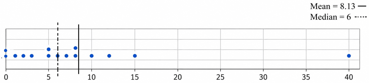
Since 8.13 > 6, the mean is indeed greater than the median, as guessed.
Hence, the mean number of short stories read is about 8.13 and the median is 6, and the mean is greater than the median.
(ii)
The value 40 is much larger than all the other observations.
Hence, 40 is the outlier.
(iii)
On removing the outlier 40, the remaining data in ascending order is:
0, 0, 1, 2, 3, 5, 5, 6, 7, 8, 8, 10, 12, 15
Mean
Sum of all observations = 0 + 0 + 1 + 2 + 3 + 5 + 5 + 6 + 7 + 8 + 8 + 10 + 12 + 15 = 82
Number of all observations = 14
Mean number of short stories =
Median
Since there are 14 observations, the median is the average of the two middle values.
Median =
After removing the outlier, the mean decreases considerably and becomes much closer to the median. The median changes only slightly. This shows that the mean is affected much more by an outlier than the median.
Do you read newspapers? Have you noticed how many pages a newspaper has on different days of the week — is it the same or different?
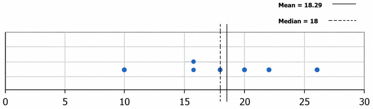
The list below shows the number of pages for a particular newspaper from Monday to Sunday: 16, 18, 20, 22, 26, 16, 10.
(i) Mark the data, the mean, and the median on the dot plot below.

Answer
Mean
Sum of all observations = 16 + 18 + 20 + 22 + 26 + 16 + 10 = 128
Number of all observations = 7
Mean number of pages =
Median
On arranging the given set of data in ascending order, we get:
10, 16, 16, 18, 20, 22, 26
There are 7 observations, so the median is the 4th value.
Median = 18
(i)
Mark the given data values on the dot plot.
Mark the mean at 18.29 and the median at 18.
Since there is no outlier in the data, the mean (18.29) and the median (18) are very close to each other.
Hence, the mean number of pages is about 18.29 and the median is 18 pages.
Discuss the effect on the mean and median when outliers are present on both sides. You may take some example data to examine and explain this.
Answer
When outliers are present on both sides, the low outlier tries to pull the mean down and the high outlier tries to pull it up. So the two effects work in opposite directions and partly cancel each other. The median, being only the middle value, is hardly affected in either case.
Example 1 — outliers roughly equally far on both sides:
Consider the data: 2, 20, 22, 24, 26, 28, 46
Here 2 is an outlier at the lower end and 46 is an outlier at the higher end. The remaining values lie between 20 and 28.
Sum of all observations = 2 + 20 + 22 + 24 + 26 + 28 + 46 = 168
Number of all observations = 7
Mean =
There are 7 observations, so the middle (4th) observation is 24.
Hence, median = 24
Since the two outliers are almost equally far from the centre, their effects cancel each other and the mean equals the median.
Example 2 — one outlier farther than the other:
Consider the data: 2, 20, 22, 24, 26, 28, 100
Sum of all observations = 2 + 20 + 22 + 24 + 26 + 28 + 100 = 222
Number of all observations = 7
Mean =
There are 7 observations, so the middle observation is 24.
Hence, median = 24
Here, the high outlier (100) is much farther from the centre than the low outlier (2). Therefore, the mean shifts towards the larger outlier, while the median remains unchanged.
Hence, when outliers are present on both sides, they pull the mean in opposite directions. If they are nearly equally far from the centre, their effects may cancel each other. If one outlier is much farther away, the mean shifts towards it. The median is affected very little in either case.
The table below shows the heights of students in a Grade 5 class in centimeters.
| Group | Heights (in cm) |
|---|---|
| Boys | 147, 135, 130, 154, 128, 135, 134, 158, 155, 146, 146, 142, 140, 141, 144, 145, 150 |
| Girls | 143, 136, 150, 144, 154, 140, 145, 148, 156, 150, 150 |
(i) How many students are taller than the class' average height?
(ii) How many boys are taller than the class’ average height?
Answer
There are 17 boys and 11 girls, so the total number of students = 17 + 11 = 28
Sum of the heights of the boys = 2430 cm
Sum of the heights of the girls = 1616 cm
Total height of all the students = 2430 + 1616 = 4046 cm
The average height of the class = = 144.5 cm
(i)
The heights greater than 144.5 cm are:
145, 145, 146, 146, 147, 148, 150, 150, 150, 150, 154, 154, 155, 156, 158
There are 15 such students.
Hence, 15 students are taller than the class' average height.
(ii)
The boys whose heights are greater than 144.5 cm are:
147, 154, 158, 155, 146, 146, 145, 150
There are 8 such boys.
Hence, 8 boys are taller than the class' average height.
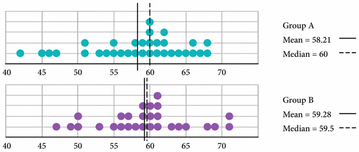
Two groups of children were asked to estimate the length of 1 minute. They start by closing their eyes and then open when they think 1 minute has passed. Of course, they are not supposed to count while their eyes are closed. The dot plots below show after how many seconds the children opened their eyes.
Discuss how well both the groups fared at this activity. Describe and compare the variability in data and their central tendency.
Answer
From the dot plots, we observe:
| Group A | Group B | |
|---|---|---|
| Number of children | 33 | 28 |
| Minimum value | 42 seconds | 47 seconds |
| Maximum value | 68 seconds | 71 seconds |
| Range | 68 - 42 = 26 seconds | 71 - 47 = 24 seconds |
| Mean | 58.21 seconds | 59.28 seconds |
| Median | 60 seconds | 59.5 seconds |
Central tendency
For both groups, the mean and the median are very close to 60 seconds. Therefore, both groups estimated one minute reasonably well.
For Group A, the mean (58.21 s) is less than the median (60 s). This shows that a few smaller values have pulled the mean down.
For Group B, the mean (59.28 s) and the median (59.5 s) are almost equal, indicating that the data are more evenly distributed about the centre.
Variability
The ranges of the two groups are very similar.
- Group B: 24 seconds
- Group A: 26 seconds
Most of the observations in both groups lie between 55 seconds and 65 seconds. Group B appears to be slightly more closely clustered around 60 seconds, indicating slightly less variability.
Hence, both groups performed well in estimating one minute. Group B estimated the time slightly better, as its mean is closer to 60 seconds and its observations are slightly less spread out than those of Group A.
Find the median of onion prices in Yahapur and Wahapur.
Answer
Yahapur:
The monthly prices (in ₹ per kg) are:
25, 24, 26, 28, 30, 35, 39, 43, 49, 56, 59, 44
Arranging them in ascending order:
24, 25, 26, 28, 30, 35, 39, 43, 44, 49, 56, 59
There are 12 observations, so the median is the average of the 6th and 7th observations.
Median =
Wahapur:
The monthly prices (in ₹ per kg) are:
19, 17, 23, 30, 38, 35, 42, 39, 53, 60, 52, 42
Arranging them in ascending order:
17, 19, 23, 30, 35, 38, 39, 42, 42, 52, 53, 60
There are 12 observations, so the median is the average of the 6th and 7th observations.
Median =
Hence, the median onion price is ₹37 per kg in Yahapur and ₹38.50 per kg in Wahapur.
Sanskruti asked her class how many domestic animals and pets each had at home. Some of the students were absent. The data values are 0, 1, 0, 4, 8, 0, 0, 2, 1, 1, 5, 3, 4, 0, 0, —, 10, 25, 2, —, 2, 4. Find the mean and median. How would you describe this data?
Answer
The dashes (—) represent students who were absent. Since they have not given any response, they are not counted as observations.
∴ The observations are:
0, 1, 0, 4, 8, 0, 0, 2, 1, 1, 5, 3, 4, 0, 0, 10, 25, 2, 2, 4
Sum of all observations = 0 + 1 + 0 + 4 + 8 + 0 + 0 + 2 + 1 + 1 + 5 + 3 + 4 + 0 + 0 + 10 + 25 + 2 + 2 + 4 = 72
Number of observations = 20
Mean =
Arranging the data in ascending order:
0, 0, 0, 0, 0, 0, 1, 1, 1, 2, 2, 2, 3, 4, 4, 4, 5, 8, 10, 25
There are 20 observations, so the median is the average of the 10th and 11th observations.
Median =
Description of the data:
Most students have 0 to 4 domestic animals or pets. The value 25 is much larger than the remaining values and is an outlier. It increases the mean, while the median is affected very little.
Hence, the mean is 3.6 and the median is 2. Since the data contains an outlier, the median represents the data better than the mean.
Rintu takes care of a date-palm tree farm in Habra. The heights of the trees (in feet) in his farm are given as: 50, 45, 43, 52, 61, 63, 46, 55, 60, 55, 59, 56, 56, 49, 54, 65, 66, 51, 44, 58, 60, 54, 52, 57, 61, 62, 60, 60, 67. Fill the dot plot, and mark the mean and median. How would you describe the heights of these palm trees? Can you think of quicker ways to find the mean? How many trees are shorter than the average height?

Answer
Sum of all observations = 50 + 45 + 43 + 52 + 61 + 63 + 46 + 55 + 60 + 55 + 59 + 56 + 56 + 49 + 54 + 65 + 66 + 51 + 44 + 58 + 60 + 54 + 52 + 57 + 61 + 62 + 60 + 60 + 67 = 1621
Number of all observations = 29
Mean =
On arranging the given set of data in ascending order, we get:
43, 44, 45, 46, 49, 50, 51, 52, 52, 54, 54, 55, 55, 56, 56, 57, 58, 59, 60, 60, 60, 60, 61, 61, 62, 63, 65, 66, 67
There are 29 observations, so the 15th observation is 56.
Hence, Median = 56 feet
Marking the mean at 55.9 feet and the median at 56 feet:

Description:
The shortest tree is 43 feet and the tallest tree is 67 feet.
The heights are mostly between 50 feet and 62 feet.
The mean (55.9 feet) and the median (56 feet) are almost equal, showing that the data are fairly balanced and do not contain any obvious outlier.
A quicker way to find the mean:
A quicker way is to add the numbers by making convenient groups or pairs so that the total can be found more easily before dividing by the number of observations.
Trees shorter than the average height:
The trees shorter than 55.9 feet are:
43, 44, 45, 46, 49, 50, 51, 52, 52, 54, 54, 55, 55
There are 13 such trees.
Hence, the mean height is about 55.9 feet, the median height is 56 feet, and 13 trees are shorter than the average height.
The daily water usage from a tap was measured. The usage in litres for the first few days is: 5.6, 8, 3.09, 12.9, 6.5, 12.1, 11.3, 20.5, 7.4.
(a) Can the mean or median daily usage lie between 25 and 30? Justify your claim using the meaning of mean and median.
(b) Can the mean or median be lesser than the minimum value or greater than the maximum value in a data?
Answer
(a)
The smallest value in the data is 3.09 litres and the largest value is 20.5 litres.
The mean represents the equal share of all the observations, so it must lie between the smallest and the largest values.
The median is the middle value of the ordered data (or the average of the two middle values), so it also lies between the smallest and the largest values.
Since 25 to 30 litres is greater than the maximum value (20.5 litres), neither the mean nor the median can lie between 25 and 30 litres.
(b)
No.
The mean always lies between the minimum and the maximum values of the data.
The median is the middle value of the ordered data (or the average of the two middle values), so it also lies between the minimum and the maximum values.
Hence, neither the mean nor the median can be less than the minimum value or greater than the maximum value of a data.
The weights of a few newborn babies are given in kgs. Fill the dot plot provided below. Analyse and compare this data.
| Boys | 3.5 | 4.1 | 2.6 | 3.2 | 3.4 | 3.8 |
|---|---|---|---|---|---|---|
| Girls | 4.0 | 3.1 | 3.4 | 3.7 | 2.5 | 3.4 |
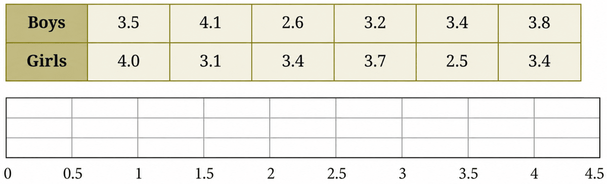
Answer
Filling the given weights on the dot plot, we get:

Boys:
Sum of all observations = 3.5 + 4.1 + 2.6 + 3.2 + 3.4 + 3.8 = 20.6
Number of all observations = 6
Mean weight =
Arranging the weights in ascending order,
2.6, 3.2, 3.4, 3.5, 3.8, 4.1
There are 6 observations, so the median is the average of the 3rd and 4th observations.
Median =
Range = 4.1 kg - 2.6 kg = 1.5 kg
Girls:
Sum of all observations = 4.0 + 3.1 + 3.4 + 3.7 + 2.5 + 3.4 = 20.1
Number of all observations = 6
Mean weight =
Arranging the weights in ascending order,
2.5, 3.1, 3.4, 3.4, 3.7, 4.0
There are 6 observations, so the median is the average of the 3rd and 4th observations.
Median =
Range = 4.0 kg - 2.5 kg = 1.5 kg
Analysis and comparison:
| Boys | Girls | |
|---|---|---|
| Minimum | 2.6 kg | 2.5 kg |
| Maximum | 4.1 kg | 4.0 kg |
| Range | 1.5 kg | 1.5 kg |
| Mean | ≈ 3.43 kg | 3.35 kg |
| Median | 3.45 kg | 3.4 kg |
The mean and the median are very close for both groups, indicating that the data are fairly balanced and there is no obvious outlier.
Both groups have the same range (1.5 kg), so the weights vary by about the same amount.
The boys have a slightly higher average weight than the girls, but the difference is very small.
Hence, the weights of the newborn boys and girls are very similar, with both groups having nearly the same spread and central tendency.
The dot plots of heights of another section of Grade 5 students of the same school are shown below. Can you share your observations? What can we infer from the dot plots and the central tendency measures?
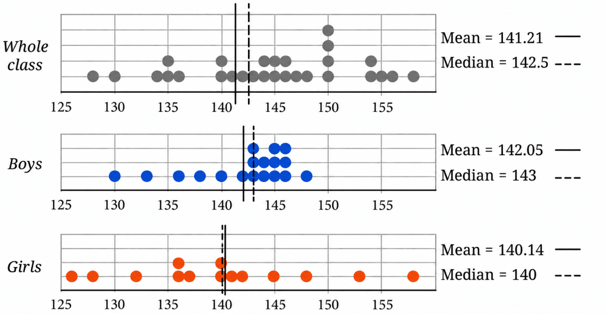
Compare the heights of the two sections. Share your observations.
Answer
Observations about this section:
From the dot plots we get:
| Whole class | Boys | Girls | |
|---|---|---|---|
| Number of students | 32 | 18 | 14 |
| Heights lie between | 126 cm and 158 cm | 130 cm and 148 cm | 126 cm and 158 cm |
| Mean | 141.21 cm | 142.05 cm | 140.14 cm |
| Median | 142.5 cm | 143 cm | 140 cm |
- The boys' heights are mostly clustered between 140 cm and 146 cm, whereas the girls' heights are spread over a wider range.
- The boys have a slightly higher mean and median than the girls.
- For all three groups, the mean and median are close to each other, indicating that the data are fairly balanced.
- There is no obvious outlier in the boys' data, while the girls' heights show a wider spread.
Comparing the two sections:
| First section | This section | |
|---|---|---|
| Number of students | 28 | 32 |
| Whole class mean | 144.4 cm | 141.21 cm |
| Whole class median | 145 cm | 142.5 cm |
| Boys' mean | 142.94 cm | 142.05 cm |
| Girls' mean | 146.9 cm | 140.14 cm |
- The first section has a higher mean and median, so its students are taller on average.
- The boys of the two sections have similar average heights.
- The girls' average height is higher in the first section than in this section.
- In the first section, the girls are slightly taller on average than the boys, whereas in this section, the boys are slightly taller on average than the girls.
- These observations apply only to these two sections and cannot be generalized to all Grade 5 students.
Hence, the first section is taller on average, while the boys of the two sections have nearly the same average height. The girls' heights show the larger difference between the two sections.
The weights of some sumo wrestlers and ballet dancers are: Sumo wrestlers: 295.2 kg, 250.7 kg, 234.1 kg, 221.0 kg, 200.9 kg. Ballet dancers: 40.3 kg, 37.6 kg, 38.8 kg, 45.5 kg, 44.1 kg, 48.2 kg. Approximately how many times heavier is a sumo wrestler compared to a ballet dancer?

Answer
To compare the two groups, we find the average weight of each group.
Total weight of sumo wrestlers = 295.2 + 250.7 + 234.1 + 221.0 + 200.9 = 1201.9
Number of wrestlers = 5
Mean weight of a sumo wrestlers =
Total weight of ballet dancers = 40.3 + 37.6 + 38.8 + 45.5 + 44.1 + 48.2 = 254.5
Number of ballet dancers = 6
Mean weight of a ballet dancers =
∴ Required number of times =
Hence, a sumo wrestler is about 5.7 times (that is, nearly 6 times) as heavy as a ballet dancer.
The two graphs can also be combined into a single graph. We just draw the bars side by side! Verify if the data in the table matches the graph below.
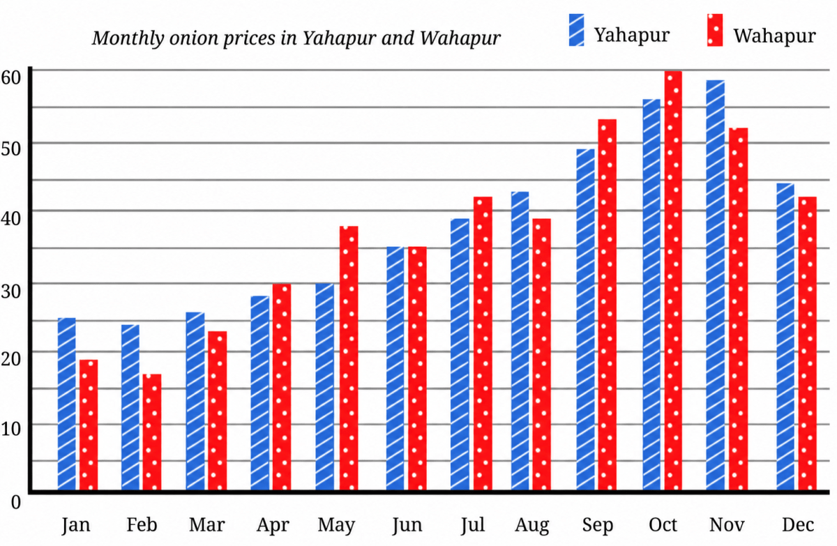
(i) What is the scale used in this graph?
(ii) Is it now easier to compare month-wise prices in both places?
Answer
Reading the heights of the bars month-wise, we find that every value shown in the graph matches the corresponding value in the table.
Hence, the data in the table matches the graph.
(i)
The horizontal axis shows the months of the year.
The vertical axis shows the price of onions (₹ per kg).
The scale used is:
- One major division = ₹10 per kg
- One smaller division = ₹5 per kg
(ii)
Yes.
Since the two bars for each month are drawn side by side, it is much easier to compare the prices in Yahapur and Wahapur.
For example:
- In January, the Yahapur bar is taller, so onions were costlier in Yahapur.
- In October, the Wahapur bar is taller, so onions were costlier in Wahapur.
- In June, both bars are of equal height, so the prices were the same.
From the graph, onions were costlier in Yahapur during 6 months, costlier in Wahapur during 5 months, and the prices were the same in June.
Hence, the clustered column graph makes month-wise comparison much easier.
Look at the graph below showing the number of worldwide rocket launches by different organisations.

(i) Identify which of the following statements can be justified using this data.
(a) All organisations launched more rockets than the previous years.
(b) Only an organisation from the USA launched more than 50 rockets in a single year.
(c) The total number of rockets launched by France in all 3 years is less than 40.
(d) The average number of rockets launched by CASC in these 3 years is around 40.
(e) ISRO launched more rockets than Galactic Energy in these 3 years.
(f) Russia launched more than 60 rockets in these 3 years.
(ii) List the organisations that have consistently launched more rockets every year.
(iii) Estimate the total number of rockets launched worldwide in 2023.
(a) less than 200
(b) 200 to 400
(c) 400 to 600
(d) more than 600
Answer
(i)
(a) This statement cannot be justified.
The number of launches by CASC fell from about 48 in 2021 to about 35 in 2022. The bars of Arianespace become shorter every year, and United Launch Alliance launched fewer rockets in 2023 than in 2022.
Hence, statement (a) cannot be justified.
(b) This statement can be justified.
SpaceX, which belongs to the USA, launched about 61 rockets in 2022 and about 96 rockets in 2023 — both more than 50. The longest bar of any other organisation is that of CASC in 2021, which is about 48, and 48 < 50.
Hence, statement (b) can be justified.
(c) This statement can be justified.
Arianespace is the organisation belonging to France. Its launches in the three years are about 15, 6 and 3.
Total number of rockets launched by France
15 + 6 + 3
= 24
As 24 < 40,
Hence, statement (c) can be justified.
(d) This statement can be justified.
The launches by CASC in the three years are about 48, 35 and 45.
Sum of all observations = 48 + 35 + 45 = 128
Number of all observations = 3
Average number of launches =
This is close to 40.
Hence, statement (d) can be justified.
(e) This statement can be justified.
Total launches by ISRO = 2 + 5 + 7 = 14
Total launches by Galactic Energy = 1 + 2 + 7 = 10
The bars of ISRO are longer than those of Galactic Energy in 2021 and in 2022, and the two are about equal in 2023. As 14 > 10,
Hence, statement (e) can be justified.
(f) This statement cannot be justified.
Roscosmos is the organisation belonging to Russia. Its launches in the three years are about 16, 21 and 18.
Total number of rockets launched by Russia
= 16 + 21 + 18
= 55
As 55 < 60,
Hence, statement (f) cannot be justified.
(ii)
An organisation has consistently launched more rockets every year if each of its bars is longer than the bar of the previous year, i.e., launches in 2021 < launches in 2022 < launches in 2023.
Checking each organisation:
| Organisation | 2021 | 2022 | 2023 | Increasing every year? |
|---|---|---|---|---|
| SpaceX | 31 | 61 | 96 | Yes |
| CASC | 48 | 35 | 45 | No |
| Roscosmos | 16 | 21 | 18 | No |
| Arianespace | 15 | 6 | 3 | No |
| Rocket Lab | 6 | 6 | 9 | No |
| United Launch Alliance | 5 | 8 | 3 | No |
| ISRO | 2 | 5 | 7 | Yes |
| Galactic Energy | 1 | 2 | 7 | Yes |
| Expace | 4 | 4 | 6 | No |
| Other | 18 | 17 | 26 | No |
Hence, the organisations that have consistently launched more rockets every year are SpaceX, ISRO and Galactic Energy.
(iii)
To estimate the total number of launches in 2023, we add the lengths of the third bar of every organisation, including the 'Other' category.
Total number of rockets launched worldwide in 2023
= 96 + 45 + 18 + 3 + 9 + 3 + 7 + 7 + 6 + 26
= 220 approximately
This lies between 200 and 400.
Hence, the correct option is (b) 200 to 400.
Answer the following questions based on the graph:
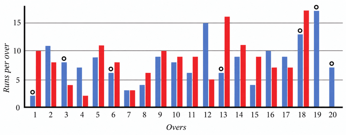
- Can we tell who batted first? Who won the match?
- How many runs did the blue team score in over 12?
- In which over did the red team score the least number of runs?
- Is it easy to tell the target set by the team batting first?
Answer
Reading the runs scored in each over from the graph (scale 1 unit = 5 runs), we get:
| Over | 1 | 2 | 3 | 4 | 5 | 6 | 7 | 8 | 9 | 10 | 11 | 12 | 13 | 14 | 15 | 16 | 17 | 18 | 19 | 20 |
|---|---|---|---|---|---|---|---|---|---|---|---|---|---|---|---|---|---|---|---|---|
| Blue team | 2 | 11 | 8 | 7 | 9 | 6 | 3 | 4 | 9 | 8 | 6 | 15 | 6 | 9 | 4 | 10 | 9 | 13 | 17 | 7 |
| Red team | 10 | 8 | 4 | 2 | 11 | 8 | 3 | 6 | 10 | 9 | 9 | 5 | 16 | 11 | 9 | 7 | 7 | 17 | — | — |
1.
No. The graph shows only the runs scored in each over by the two teams. It does not indicate which team batted first or which team won the match.
Although the blue team has a total of about 163 runs and the red team has about 152 runs, the graph alone does not state the order of innings or the match result.
Hence, from the graph alone, we cannot tell who batted first or who won the match.
2.
The blue bar for over 12 reaches 15 runs.
Hence, the blue team scored 15 runs in over 12.
3.
The shortest red bar is in over 4, where the team scored 2 runs.
Hence, the red team scored the least number of runs, i.e., 2 runs, in over 4.
4.
No. The graph shows the runs scored in each over, not the cumulative score. To find the target, we would have to read the runs scored in every over by the team batting first and add them.
Hence, it is not easy to tell the target directly from the graph.
The following infographic shows the speeds of a few animals in air, on land, and in water. Can we call this graph a bar graph?
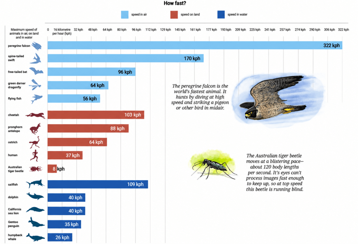
(a) What is the scale used in this graph?
(b) What did you find interesting in this infographic? What do you want to explore further?
(c) Identify a pair of creatures where one's speed is about twice that of the other.
(d) Can we say that a sailfish is about 4 times faster than a humpback whale? Can we say that a sailfish is the fastest aquatic animal in the world?
Answer
Yes. This infographic can be called a bar graph.
Each creature is represented by a bar whose length shows its maximum speed. The colours are used only to distinguish creatures that move in air, on land, and in water. The pictures make the graph attractive but do not change the type of graph.
(a)
The horizontal axis is marked
0, 16, 32, 48, 64, 80, 96, …
The difference between two consecutive markings is 16 kilometres per hour (km/h).
Hence, the scale used is one major division = 16 km/h.
(b) Some interesting observations from the infographic are:
- The peregrine falcon, at 322 km/h, is the fastest creature among those shown and is nearly twice as fast as the spine-tailed swift at 170 km/h.
- The sailfish, at 109 km/h, is slightly faster than the cheetah at 103 km/h.
- The Australian tiger beetle has a much lower speed in km/h, but the note explains that it can cover about 120 body lengths per second.
Some questions that may be explored further are:
- For how long can the different creatures maintain their maximum speeds?
- Which creature is fastest when speed is compared in body lengths per second?
- How would other animals compare with the creatures shown in the infographic?
(c)
For example,
Speed of the peregrine falcon = 322 km/h
Speed of the spine-tailed swift = 170 km/h
So, the peregrine falcon is about twice as fast as the spine-tailed swift.
Another example is:
Speed of the sailfish = 109 km/h
Speed of the flying fish = 56 km/h
So, the sailfish is about twice as fast as the flying fish.
Hence, suitable pairs are the peregrine falcon and spine-tailed swift, or the sailfish and flying fish.
(d)
Speed of the sailfish = 109 km/h
Speed of the humpback whale = 26 km/h
So, yes, a sailfish is about 4 times faster than a humpback whale.
However, no, we cannot say that the sailfish is the fastest aquatic animal in the world. The infographic shows only a few selected aquatic animals. It does not include every aquatic animal, so such a conclusion cannot be drawn.
Hence, a sailfish is about four times faster than a humpback whale, but we cannot conclude from this infographic that it is the fastest aquatic animal in the world.
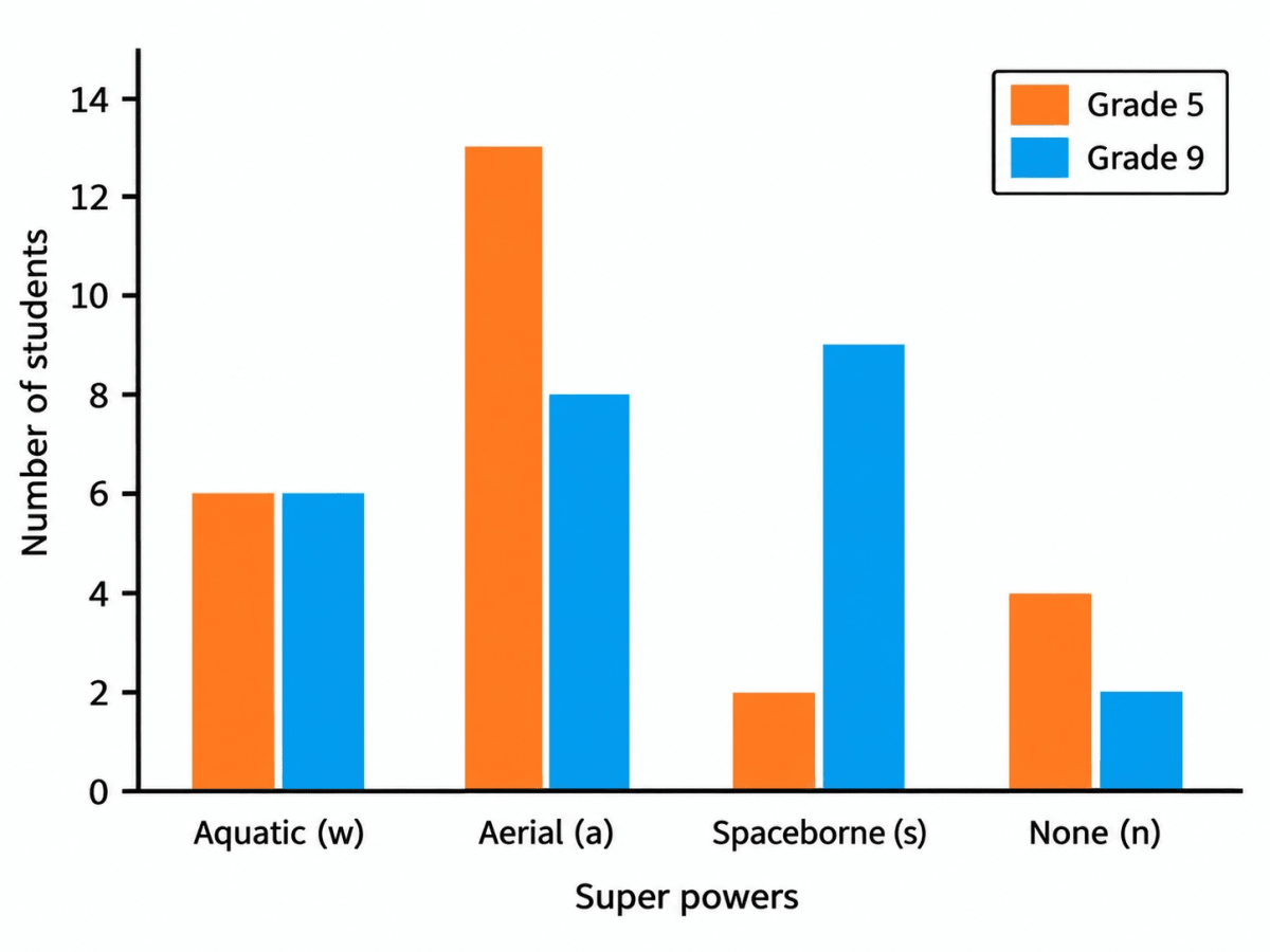
Preyashi asked her students 'If you were to get a super power to become aquatic (water-borne), aerial (air-borne), or spaceborne which one would you choose?'. The responses are shown below. Some chose none. Draw a double-bar graph comparing how both grades chose each option. Choose an appropriate scale.
| Grade 5 | w, a, a, a, w, n, s, a, n, w, a, a, a, a, a, w, w, s, a, a, n, w, a, a, n |
|---|---|
| Grade 9 | n, w, s, a, s, w, s, s, a, a, w, s, s, a, s, a, n, w, s, s, a, w, a, w, a |
Answer
Counting how many times each letter occurs in each row, we get the following frequency table:
| Super power | Grade 5 | Grade 9 |
|---|---|---|
| Aquatic (w) | 6 | 6 |
| Aerial (a) | 13 | 8 |
| Spaceborne (s) | 2 | 9 |
| None (n) | 4 | 2 |
| Total | 25 | 25 |
Choose a convenient scale.
Scale: 1 unit = 2 students
Draw a double bar graph with:
- Horizontal axis: Super powers
- Vertical axis: Number of students
- Two bars of different colours for each category, one representing Grade 5 and the other Grade 9.
Observations from the graph:
Aerial is the most preferred super power in Grade 5, chosen by 13 students.
Spaceborne is the most preferred super power in Grade 9, chosen by 9 students.
Aquatic is chosen by 6 students in both grades.
None is chosen by 4 students in Grade 5 and 2 students in Grade 9.
Hence, the double bar graph compares the choices of students in Grade 5 and Grade 9 using the scale 1 unit = 2 students.
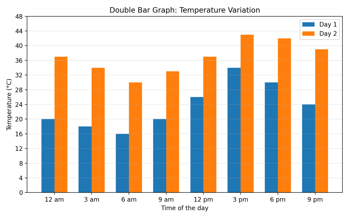
The temperature variation over two days in different months in Jodhpur, Rajasthan, is given below. Draw a double-bar graph. Use the scale 1 unit = 4°C. Can you guess which two months these days might belong to?
| 12 am | 3 am | 6 am | 9 am | 12 pm | 3 pm | 6 pm | 9 pm | |
|---|---|---|---|---|---|---|---|---|
| Day 1 | 20°C | 18°C | 16°C | 20°C | 26°C | 34°C | 30°C | 24°C |
| Day 2 | 37°C | 34°C | 30°C | 33°C | 37°C | 43°C | 42°C | 39°C |
Answer
Draw a double bar graph using:
- Horizontal axis: Time of the day
- Vertical axis: Temperature (°C)
- Scale: 1 unit = 4°C
Draw two bars of different colours side by side for each time.
From the graph, we observe that:
- On Day 1, the temperature varies from 16°C to 34°C.
- On Day 2, the temperature varies from 30°C to 43°C.
- The temperature is lowest in the early morning and highest in the afternoon on both days.
Since Day 2 remains very hot throughout the day, it could belong to a summer month such as May or June.
Since Day 1 has comparatively cooler temperatures, it could belong to a month such as March or October–November.
Hence, the double bar graph is as drawn above. Day 1 may belong to March (or October–November), while Day 2 may belong to May or June.
The following clustered-bar graph shows the number of electric vehicles registered in some states every year from 2022 to 2024.
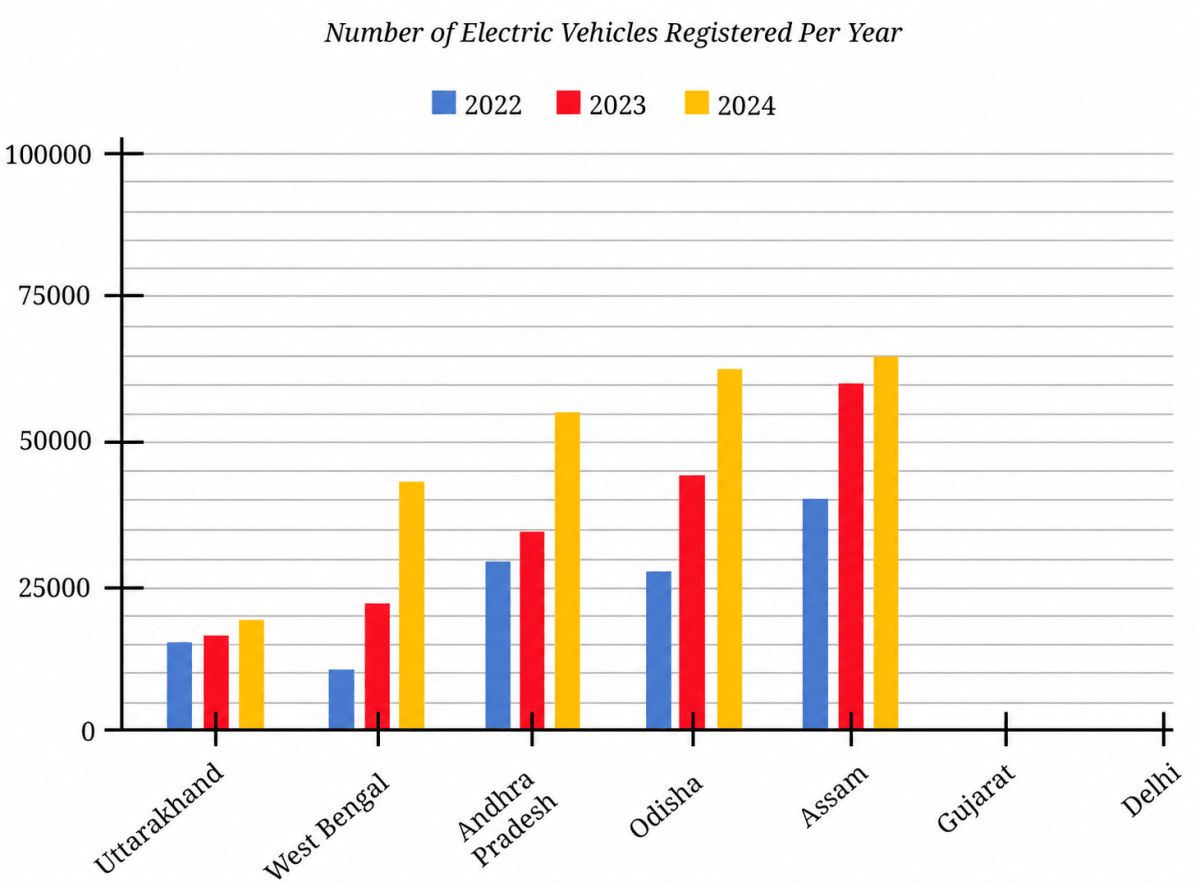
(a) The data (rounded-off to thousands) for the states of Gujarat and Delhi are given in the table below. Mark the corresponding bars on the bar graph. (It is enough if you place the top of the bars between the two appropriate vertical guidelines.)
| 2022 | 2023 | 2024 | |
|---|---|---|---|
| Gujarat | 69000 | 89000 | 78000 |
| Delhi | 62000 | 74000 | 81000 |
(b) Notice how the graph is organised, what scale is used, and what patterns the data shows.
(c) How would you describe the change for various states between 2022 and 2024?
(d) Approximately how many more registrations did Assam get in 2023 compared to 2022?
(e) How many times more did the registrations in West Bengal increase from 2022 to 2024?
(f) Is this statement correct — 'There were very few new registrations in Uttarakhand in 2023 and 2024, as the increase in the bar lengths is minimal'?
Answer
(a)
The graph has horizontal guidelines at intervals of 5000 registrations.
The six bars should be drawn with their tops at the following approximate heights:
| Bar | Value | Top of the bar lies between |
|---|---|---|
| Gujarat 2022 | 69000 | 65000 and 70000 |
| Gujarat 2023 | 89000 | 85000 and 90000 |
| Gujarat 2024 | 78000 | 75000 and 80000 |
| Delhi 2022 | 62000 | 60000 and 65000 |
| Delhi 2023 | 74000 | 70000 and 75000 |
| Delhi 2024 | 81000 | 80000 and 85000 |
Marking these six bars in the empty spaces kept for Gujarat and Delhi, and using the same three colours as the other states, we get :
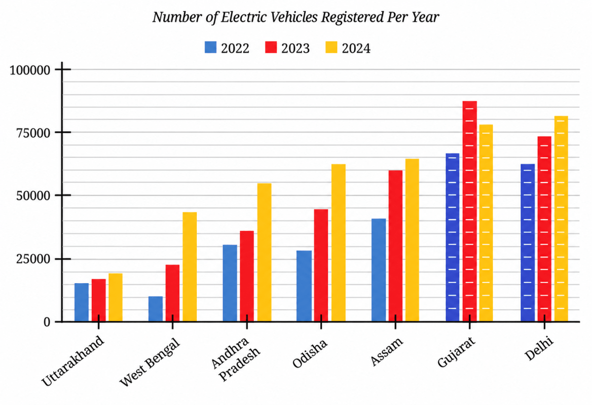
Hence, the six bars are drawn as shown above, with the tops of the Gujarat bars a little below 70000, a little below 90000 and a little below 80000, and the tops of the Delhi bars a little above 60000, a little below 75000 and a little above 80000.
(b)
- The horizontal axis shows the states and the vertical axis shows the number of electric vehicles registered.
- The labelled marks are 0, 25000, 50000, 75000 and 100000. There are five equal smaller divisions in each interval of 25000, so one small division represents about 5000 registrations.
- Each state has three adjacent bars representing 2022, 2023 and 2024.
- Uttarakhand, West Bengal, Andhra Pradesh, Odisha, Assam and Delhi show an overall increase across the period. Gujarat increases from 2022 to 2023 and then decreases in 2024, though its 2024 value is still greater than its 2022 value.
(c)
Comparing 2022 with 2024, registrations increased in all the states shown. From the graph, the approximate increases for the first five states are:
- Uttarakhand: about 4000
- West Bengal: about 33000
- Andhra Pradesh: about 26000
- Odisha: about 35000
- Assam: about 24000
For the given values, Gujarat increases by 9000 and Delhi by 19000.
Thus, Odisha shows the largest approximate increase from 2022 to 2024, while Uttarakhand shows the smallest increase.
Hence, all the states show an overall increase from 2022 to 2024, although Gujarat rises sharply in 2023 and then falls in 2024.
(d) From the graph,
Registrations in Assam in 2022 ≈ 40000
Registrations in Assam in 2023 ≈ 60000
Difference: 60000 − 40000 = 20000
Hence, Assam got about 20000 more registrations in 2023 as compared to 2022.
(e) From the graph,
West Bengal registrations in 2022 ≈ 10000
West Bengal registrations in 2024 ≈ 43000
=
Hence, the registrations in West Bengal increased to about 4 times the 2022 registrations by 2024.
(f) No. A small increase in bar length means that the increase in registrations was small. It does not mean that the total number of registrations in those years was very small.
Hence, the statement is not correct; the graph shows a small increase in Uttarakhand, not an absence of registrations.
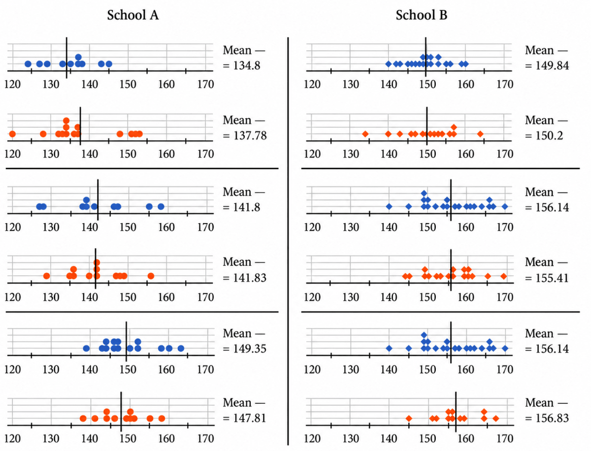
Following are the dot plots of heights of boys (in blue) and girls (in orange) of Grades 6, 7 and 8 (in that order) of two different schools. What do you notice? Share your observations.
Answer
The means marked on the dot plots are:
| Grade | School A — Boys | School A — Girls | School B — Boys | School B — Girls |
|---|---|---|---|---|
| Grade 6 | 134.8 cm | 137.78 cm | 149.84 cm | 150.2 cm |
| Grade 7 | 141.8 cm | 141.83 cm | 156.14 cm | 155.41 cm |
| Grade 8 | 149.35 cm | 147.81 cm | 156.14 cm | 156.83 cm |
Observations:
- In every grade, the mean heights of both boys and girls are higher in School B than in School A.
- In both schools, the mean heights generally increase from Grade 6 to Grade 8.
- The difference between boys' and girls' mean heights within the same grade is small compared with the difference between the two schools.
- In School A, girls have a slightly higher mean in Grades 6 and 7, while boys have a higher mean in Grade 8. In School B, girls have a slightly higher mean in Grades 6 and 8, while boys have a slightly higher mean in Grade 7.
- The mean height of Grade 6 students in School B is close to, and in some cases slightly greater than, the mean height of Grade 8 students in School A.
- The dot plots show a clear difference between the two schools, but the data alone does not tell us the reason for this difference. More information would be needed before drawing any conclusion about its cause.
These are different groups of students, so differences between grades should not be treated as measurements of how the same children grew over time.
Hence, School B has higher mean heights in all three grades, while the differences between boys and girls within a grade are comparatively small.
Spend sufficient time observing the data presented in this table. Share your findings with the class.
| Age | 1989 | 1999 | 2009 | 2019 | ||||
|---|---|---|---|---|---|---|---|---|
| 5 | 101.3 | 100 | 102.4 | 101.7 | 105.1 | 104 | 107.1 | 107.2 |
| 6 | 107.5 | 106 | 108.7 | 107.5 | 111 | 109.7 | 113.1 | 112.9 |
| 7 | 113 | 111.4 | 114.2 | 112.6 | 116.2 | 114.8 | 118.6 | 118 |
| 8 | 118.1 | 116.5 | 119.2 | 117.5 | 120.9 | 119.6 | 123.5 | 122.7 |
| 9 | 122.9 | 121.7 | 123.9 | 122.4 | 125.2 | 124.5 | 128.1 | 127.6 |
| 10 | 127.5 | 127.3 | 128.3 | 127.8 | 129.4 | 129.9 | 132.6 | 132.8 |
| 11 | 132.2 | 133.4 | 132.8 | 133.6 | 133.7 | 135.7 | 137 | 138.6 |
| 12 | 137.7 | 139 | 138 | 139.1 | 138.9 | 141.1 | 142.2 | 143.8 |
| 13 | 144.2 | 143.2 | 144.3 | 143.1 | 145.2 | 145.1 | 148.4 | 147.7 |
| 14 | 150.6 | 146.2 | 150.5 | 146.1 | 151.5 | 148 | 154.4 | 150.4 |
| 15 | 155.4 | 148.5 | 155.2 | 148.4 | 156.3 | 150.1 | 159 | 152.4 |
| 16 | 158.9 | 150.1 | 158.7 | 150.1 | 159.9 | 151.6 | 162.3 | 153.8 |
| 17 | 161.3 | 151.2 | 161.4 | 151.3 | 162.6 | 152.6 | 164.6 | 154.7 |
| 18 | 162.9 | 151.8 | 163.2 | 152.1 | 164.3 | 153 | 166 | 155.2 |
| 19 | 163.5 | 151.9 | 164.2 | 152.4 | 165.1 | 153 | 166.5 | 155.2 |
(i) These are some prompts for you to probe —
- Changes in the heights of boys or girls of a certain age from 1989 to 2019.
- The heights of boys vs. girls at different ages in a particular year.
- Changes in height between successive ages in boys and girls in 2019.
(ii) Which of the following statements can be justified using the data?
- The average heights of both boys and girls at every age increased from 1989 to 2019.
- The average height of 13-year-old girls in 1989 is more than the average height of 14-year-old girls in 2009.
- The average height of 15-year-old boys in 2019 is more than the average height of 16-year-old boys in 1989.
- All girls aged 13 are taller than all girls aged 11.
- Throughout the age period 5 to 19, the average boy's height is more than the average girl's height.
- Boys keep growing even beyond age 19.
(iii) In 2019, between which two successive ages from 5 to 19 did boys grow the most? Between which two successive ages from 5 to 19 did girls grow most?
(iv) Suppose the average height of a newborn is 50 cm. Estimate the average height of young children of ages 1 to 4.
(v) Based on the trend observed in the table, write your estimates of the heights of boys and girls for ages 5 to 19 in the year 2029.
Answer
The following table shows the average heights of boys and girls (in centimeters) across ages 5 to 19 in the years 1989, 1999, 2009, and 2019. In each year, the first column shows boys' heights and the second column shows girls' heights.
Prompt 1 — Changes from 1989 to 2019 at a given age.
Subtracting the 1989 height from the 2019 height at each age, we get:
| Age | Increase in boys' height (cm) | Increase in girls' height (cm) |
|---|---|---|
| 5 | 5.8 | 7.2 |
| 6 | 5.6 | 6.9 |
| 7 | 5.6 | 6.6 |
| 8 | 5.4 | 6.2 |
| 9 | 5.2 | 5.9 |
| 10 | 5.1 | 5.5 |
| 11 | 4.8 | 5.2 |
| 12 | 4.5 | 4.8 |
| 13 | 4.2 | 4.5 |
| 14 | 3.8 | 4.2 |
| 15 | 3.6 | 3.9 |
| 16 | 3.4 | 3.7 |
| 17 | 3.3 | 3.5 |
| 18 | 3.1 | 3.4 |
| 19 | 3.0 | 3.3 |
From this table we observe that:
At every single age from 5 to 19, the average height in 2019 is more than that in 1989, for both boys and girls. Over these 30 years, children of the same age have become taller.
The gain is largest at the younger ages and steadily becomes smaller as the age increases. For example, 5-year-old boys gained 5.8 cm while 19-year-old boys gained only 3.0 cm.
At every age the girls' gain is more than the boys' gain. For instance, at age 5 the girls gained 7.2 cm against the boys' 5.8 cm.
Prompt 2 — Boys vs. girls at different ages in 2019.
Subtracting the girls' height from the boys' height for each age in 2019, we get:
| Age | 5 | 6 | 7 | 8 | 9 | 10 | 11 | 12 | 13 | 14 | 15 | 16 | 17 | 18 | 19 |
|---|---|---|---|---|---|---|---|---|---|---|---|---|---|---|---|
| Boys – Girls (cm) | –0.1 | 0.2 | 0.6 | 0.8 | 0.5 | –0.2 | –1.6 | –1.6 | 0.7 | 4.0 | 6.6 | 8.5 | 9.9 | 10.8 | 11.3 |
From this table we observe that:
Between ages 6 and 9 the boys are taller, but only by a very small amount (at most 0.8 cm).
At ages 10, 11 and 12 the girls are on average taller than the boys, the difference being the largest (1.6 cm) at ages 11 and 12.
From age 13 onwards the boys are again taller, and the gap now widens rapidly, reaching 11.3 cm at age 19.
Prompt 3 — Change between successive ages in 2019.
Subtracting the height at one age from the height at the next age in 2019, we get:
| From age → to age | Boys' growth (cm) | Girls' growth (cm) |
|---|---|---|
| 5 → 6 | 6.0 | 5.7 |
| 6 → 7 | 5.5 | 5.1 |
| 7 → 8 | 4.9 | 4.7 |
| 8 → 9 | 4.6 | 4.9 |
| 9 → 10 | 4.5 | 5.2 |
| 10 → 11 | 4.4 | 5.8 |
| 11 → 12 | 5.2 | 5.2 |
| 12 → 13 | 6.2 | 3.9 |
| 13 → 14 | 6.0 | 2.7 |
| 14 → 15 | 4.6 | 2.0 |
| 15 → 16 | 3.3 | 1.4 |
| 16 → 17 | 2.3 | 0.9 |
| 17 → 18 | 1.4 | 0.5 |
| 18 → 19 | 0.5 | 0.0 |
From this table we observe that:
Both boys and girls show a spurt of fast growth, but the girls' spurt comes earlier (around ages 10 to 12) than the boys' spurt (around ages 12 to 14).
After the spurt the yearly growth falls steadily for both. The girls have practically stopped growing between 18 and 19 (0.0 cm), while the boys are still growing a little (0.5 cm).
This earlier spurt of the girls is exactly what makes them taller than the boys at ages 10, 11 and 12, and the boys' later and longer spurt is what puts them well ahead from age 13 onwards.
Hence, over 1989 – 2019 children of every age have grown taller (girls gaining slightly more than boys), girls overtake boys in average height for the short period of ages 10 to 12 because their growth spurt comes earlier, and boys move far ahead after age 13.
(ii)
Statement 1: The average heights of both boys and girls at every age increased from 1989 to 2019.
Comparing the 1989 column with the 2019 column at each age, we find that the height increases at every one of the 15 ages, for boys as well as for girls. The smallest of these increases is 3.0 cm (boys aged 19) and the largest is 7.2 cm (girls aged 5), and all of them are positive.
Hence, Statement 1 can be justified using the data. It is true.
Statement 2: The average height of 13-year-old girls in 1989 is more than the average height of 14-year-old girls in 2009.
Average height of 13-year-old girls in 1989 = 143.2 cm
Average height of 14-year-old girls in 2009 = 148 cm
Since 143.2 < 148, the first value is in fact less than the second.
Hence, Statement 2 cannot be justified using the data. It is false.
Statement 3: The average height of 15-year-old boys in 2019 is more than the average height of 16-year-old boys in 1989.
Average height of 15-year-old boys in 2019 = 159 cm
Average height of 16-year-old boys in 1989 = 158.9 cm
Since 159 > 158.9, the first value is more than the second.
Hence, Statement 3 can be justified using the data. It is true.
Statement 4: All girls aged 13 are taller than all girls aged 11.
The table gives only the average height of all the girls of a particular age. An average tells us nothing about any one individual girl — some 13-year-old girls will be shorter than the average and some 11-year-old girls will be taller than the average. So the table cannot tell us anything about all girls.
Hence, Statement 4 cannot be justified using the data.
Statement 5: Throughout the age period 5 to 19, the average boy's height is more than the average girl's height.
At age 11, in every one of the four years the girls' average is more than the boys':
The same happens at age 12 in all four years, at age 10 in 2009 and 2019, and at age 5 in 2019.
Hence, Statement 5 cannot be justified using the data. It is false.
Statement 6: Boys keep growing even beyond age 19.
The table stops at age 19. It contains no information at all about heights at age 20 or beyond, so nothing can be concluded about growth after age 19 from this data.
Hence, Statement 6 cannot be justified using the data.
(iii)
To find the growth between two successive ages, we subtract the height at the lower age from the height at the next higher age, using the 2019 columns.
| From age → to age | Boys' growth (cm) | Girls' growth (cm) |
|---|---|---|
| 5 → 6 | 6.0 | 5.7 |
| 6 → 7 | 5.5 | 5.1 |
| 7 → 8 | 4.9 | 4.7 |
| 8 → 9 | 4.6 | 4.9 |
| 9 → 10 | 4.5 | 5.2 |
| 10 → 11 | 4.4 | 5.8 |
| 11 → 12 | 5.2 | 5.2 |
| 12 → 13 | 6.2 | 3.9 |
| 13 → 14 | 6.0 | 2.7 |
| 14 → 15 | 4.6 | 2.0 |
| 15 → 16 | 3.3 | 1.4 |
| 16 → 17 | 2.3 | 0.9 |
| 17 → 18 | 1.4 | 0.5 |
| 18 → 19 | 0.5 | 0.0 |
For the boys, the largest value in the growth column is 6.2 cm, which occurs between the ages of 12 and 13.
148.4 - 142.2 = 6.2 cm
For the girls, the largest value in the growth column is 5.8 cm, which occurs between the ages of 10 and 11.
138.6 - 132.8 = 5.8 cm
Hence, in 2019 the boys grew the most between the ages of 12 and 13 (6.2 cm), and the girls grew the most between the ages of 10 and 11 (5.8 cm).
(iv)
The table does not give heights for ages 1 to 4, so there is no single exact answer. One simple estimate is to use the given average height of a newborn (50 cm) and the average height at age 5 in 2019 (about 107 cm), and assume an approximately equal increase over these five years.
Total increase from birth to age 5
= 107 cm - 50 cm
= 57 cm
Approximate increase per year
One possible set of estimates is therefore:
| Age | 1 | 2 | 3 | 4 |
|---|---|---|---|---|
| Estimated average height | 61.4 cm | 72.8 cm | 84.2 cm | 95.6 cm |
These are only estimates; different reasonable methods may give somewhat different values.
Hence, one possible estimate is about 61 cm, 73 cm, 84 cm and 96 cm for ages 1, 2, 3 and 4, respectively.
(v)
The most recent decade in the table is 2009 to 2019. Assuming that the heights change over 2019 – 2029 by the same amount as they changed over 2009 – 2019, we add the 2009 → 2019 increase to the 2019 height at each age.
For example, for 5-year-old boys:
Increase from 2009 to 2019 = 107.1 - 105.1 = 2 cm
Estimate for 2029 = 107.1 + 2 = 109.1 cm
Repeating this for every age, we get the following estimates.
| Age | Boys 2019 | Increase | Boys 2029 | Girls 2019 | Increase | Girls 2029 |
|---|---|---|---|---|---|---|
| 5 | 107.1 | 2.0 | 109.1 | 107.2 | 3.2 | 110.4 |
| 6 | 113.1 | 2.1 | 115.2 | 112.9 | 3.2 | 116.1 |
| 7 | 118.6 | 2.4 | 121.0 | 118.0 | 3.2 | 121.2 |
| 8 | 123.5 | 2.6 | 126.1 | 122.7 | 3.1 | 125.8 |
| 9 | 128.1 | 2.9 | 131.0 | 127.6 | 3.1 | 130.7 |
| 10 | 132.6 | 3.2 | 135.8 | 132.8 | 2.9 | 135.7 |
| 11 | 137.0 | 3.3 | 140.3 | 138.6 | 2.9 | 141.5 |
| 12 | 142.2 | 3.3 | 145.5 | 143.8 | 2.7 | 146.5 |
| 13 | 148.4 | 3.2 | 151.6 | 147.7 | 2.6 | 150.3 |
| 14 | 154.4 | 2.9 | 157.3 | 150.4 | 2.4 | 152.8 |
| 15 | 159.0 | 2.7 | 161.7 | 152.4 | 2.3 | 154.7 |
| 16 | 162.3 | 2.4 | 164.7 | 153.8 | 2.2 | 156.0 |
| 17 | 164.6 | 2.0 | 166.6 | 154.7 | 2.1 | 156.8 |
| 18 | 166.0 | 1.7 | 167.7 | 155.2 | 2.2 | 157.4 |
| 19 | 166.5 | 1.4 | 167.9 | 155.2 | 2.2 | 157.4 |
These estimates keep all the features seen in the earlier data — the girls are estimated to be taller than the boys at ages 11 and 12, the boys move ahead from age 13, and the difference at age 19 is about 10.5 cm.
Hence, in 2029 the average height of boys is estimated to rise from about 109 cm at age 5 to about 168 cm at age 19, and that of girls from about 110 cm at age 5 to about 157 cm at age 19.
The dot plots below show the distribution of the number of pockets on clothing for a group of boys and for a group of girls.
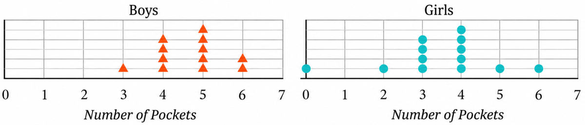
Based on the dot plots, which of the following statements are true?
(a) The data varies more for the boys than for the girls.
(b) The median number of pockets for the boys is more than that for the girls.
(c) The mean number of pockets for the girls is more than that for the boys.
(d) The maximum number of pockets for boys is greater than that for the girls.
Answer
Reading the dots from the two dot plots, we get:
| Number of pockets | 0 | 1 | 2 | 3 | 4 | 5 | 6 | 7 |
|---|---|---|---|---|---|---|---|---|
| Number of boys | 0 | 0 | 0 | 1 | 4 | 5 | 2 | 0 |
| Number of girls | 1 | 0 | 1 | 4 | 5 | 1 | 1 | 0 |
Boys : 3, 4, 4, 4, 4, 5, 5, 5, 5, 5, 6, 6
Girls : 0, 2, 3, 3, 3, 3, 4, 4, 4, 4, 4, 5, 6
There are 12 observations for the boys and 13 observations for the girls.
(a) The data varies more for the boys than for the girls.
Range of boys' data = Highest observation - Lowest observation
= 6 - 3
= 3
Range of girls' data = Highest observation - Lowest observation
= 6 - 0
= 6
Since 6 > 3, the girls' data is more spread out than the boys' data.
Hence, statement (a) is false.
(b) The median number of pockets for the boys is more than that for the girls.
Median (boys):
6th and 7th terms are both 5.
Median = 5
Median (girls):
There are 13 values for the girls. The median is the 7th value:
Median = 4
Since 5 > 4, the median for the boys is more than that for the girls.
Hence, statement (b) is true.
(c) The mean number of pockets for the girls is more than that for the boys.
For boys:
Sum of all observations = 3 + 4 + 4 + 4 + 4 + 5 + 5 + 5 + 5 + 5 + 6 + 6 = 56
Number of all observations = 12
Mean =
For girls:
Sum of all observations = 0 + 2 + 3 + 3 + 3 + 3 + 4 + 4 + 4 + 4 + 4 + 5 + 6 = 45
Number of all observations = 13
Mean =
Since 3.46 < 4.67, the mean for the girls is less than that for the boys.
Hence, statement (c) is false.
(d) The maximum number of pockets for boys is greater than that for the girls.
Maximum number of pockets for boys = 6
Maximum number of pockets for girls = 6
Since 6 = 6, the maximum for the boys is equal to, and not greater than, the maximum for the girls.
Hence, statement (d) is false.
The following table shows the points scored by each player in four games:
| Player | Game 1 | Game 2 | Game 3 | Game 4 |
|---|---|---|---|---|
| A | 14 | 16 | 10 | 10 |
| B | 0 | 8 | 6 | 4 |
| C | 8 | 11 | Did not play | 13 |
Now answer the following questions:
(a) Find the average number of points scored per game by A.
(b) To find the mean number of points scored per game by C, would you divide the total points by 3 or by 4? Why? What about B?
(c) Who is the best performer?
Answer
(a) A played all 4 games.
Sum of all observations = 14 + 16 + 10 + 10 = 50
Number of all observations = 4
Average points scored per game by A =
Hence, the average number of points scored per game by A is 12.5.
(b) C did not play Game 3. So there is no value for C in Game 3 — it is a blank, not a score. C actually played only 3 games, and so the total must be divided by 3.
Sum of all observations = 8 + 11 + 13 = 32
Number of all observations = 3
Mean points scored per game by C =
B is different. B played all 4 games and scored 0 points in Game 1. Here 0 is a value — it records that B played and did not score. So for B the total must be divided by 4.
Sum of all observations = 0 + 8 + 6 + 4 = 18
Number of all observations = 4
Mean points scored per game by B =
Hence, for C we divide by 3 because C played only 3 games, whereas for B we divide by 4 because B played all 4 games and 0 is a score, not a missing value.
(c) Comparing the average points scored per game by the three players:
A = 12.5, C = 10.67 (approx.), B = 4.5
Since 12.5 > 10.67 > 4.5, A has the highest average. A also has the highest total (50 points) and scored 10 or more points in every game.
Hence, A is the best performer.
The marks (out of 100) obtained by a group of students in a General Knowledge quiz are 85, 76, 90, 85, 39, 48, 56, 95, 81 and 75. Another group's scores in the same quiz are 68, 59, 73, 86, 47, 79, 90, 93 and 86. Compare and describe both the groups performance using, mean and median.
Answer
Group 1
Sum of all observations = 85 + 76 + 90 + 85 + 39 + 48 + 56 + 95 + 81 + 75 = 730
Number of all observations = 10
Mean =
Arrange the marks in ascending order:
39, 48, 56, 75, 76, 81, 85, 85, 90, 95
There are 10 observations.
The two middle observations are the 5th and 6th observations, namely 76 and 81.
Median =
Group 2
Sum of all observations = 68 + 59 + 73 + 86 + 47 + 79 + 90 + 93 + 86 = 681
Number of all observations = 9
Mean =
Arrange the marks in ascending order:
47, 59, 68, 73, 79, 86, 86, 90, 93
There are 9 observations.
The middle (5th) observation is 79.
Therefore, median = 79
Comparison
| Group 1 | Group 2 | |
|---|---|---|
| Mean | 73 | 75.67 (approx.) |
| Median | 78.5 | 79 |
| Lowest mark | 39 | 47 |
| Highest mark | 95 | 93 |
| Range | 56 | 46 |
From the above results, we observe that:
- The mean of Group 2 (75.67) is greater than that of Group 1 (73).
- The median of Group 2 (79) is also slightly greater than that of Group 1 (78.5).
- In both the groups, the mean is less than the median, showing that the lower marks reduce the mean.
- The difference between the mean and the median is greater for Group 1, indicating that the lower marks have a greater effect on its mean.
Hence, Group 2 performed slightly better than Group 1 because both its mean and median are higher than those of Group 1.
Consider this data collected from a survey of a colony.
| Favourite Sport | Cricket | Basket Ball | Swimming | Hockey | Athletics |
|---|---|---|---|---|---|
| Watching | 1240 | 470 | 510 | 430 | 250 |
| Participating | 620 | 320 | 320 | 250 | 105 |
Choose an appropriate scale and draw a double-bar graph. Write down your observations.
Answer
The greatest value in the table is 1240. Hence, a suitable scale is
Scale: 1 unit = 100 people
Draw a double-bar graph with:
- Favourite sports along the horizontal axis.
- Number of people along the vertical axis.
- Two bars for each sport:
- one representing Watching,
- the other representing Participating.
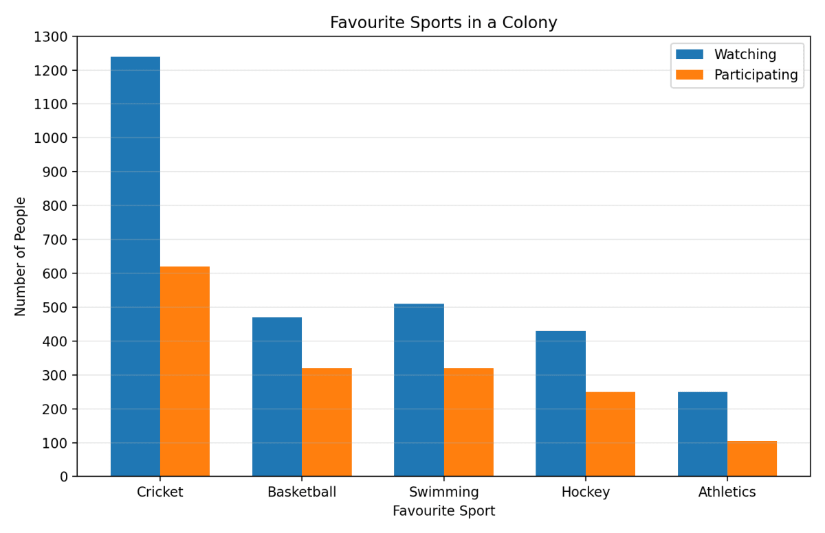
Observations:
- Cricket is the most popular sport both for watching (1240 people) and participating (620 people).
- Athletics is the least popular sport in both categories.
- For every sport, the number of people who watch the sport is greater than the number of people who participate in it.
- The number of people watching cricket is exactly twice the number of people participating in it.
- Basketball and swimming have the same number of participants (320 each), but more people prefer watching swimming (510) than basketball (470).
Hence, cricket is the most popular sport in the colony, athletics is the least popular, and for every sport more people prefer watching than participating.
Consider a group of 17 students with the following heights (in cm): 106, 110, 123, 125, 117, 120, 112, 115, 110, 120, 115, 102, 115, 115, 109, 115, 101. The sports teacher wants to divide the class into two groups so that each group has an equal number of students: one group has students with height less than a particular height and the other group has students with heights greater than the particular height. Suggest a way to do this. Can you guess the age of these students based on the tabular data in the 'Telling Tall Tales' section?
Answer
Arrange the heights in ascending order:
101, 102, 106, 109, 110, 110, 112, 115, 115, 115, 115, 115, 117, 120, 120, 123, 125
There are 17 observations.
Since the number of observations is odd, the middle (9th) observation is 115 cm.
Therefore, the median height is 115 cm.
The teacher can use 115 cm as the dividing height.
Students with height less than 115 cm:
101, 102, 106, 109, 110, 110, 112
→ 7 studentsStudents with height equal to 115 cm:
115, 115, 115, 115, 115
→ 5 studentsStudents with height greater than 115 cm:
117, 120, 120, 123, 125
→ 5 students
Since there are 17 students, it is not possible to divide them into two groups having exactly the same number of students. The teacher may place one student of height 115 cm with the shorter group and the remaining four students of height 115 cm with the taller group. This gives two groups of 8 and 9 students.
From the 'Telling Tall Tales' table, a typical height of about 115 cm corresponds approximately to children of 6–7 years of age.
Hence, the teacher can use the median height, 115 cm, as the dividing height, and the students are likely to be about 6–7 years old.
There are two 7th grade sections at a school. Each section has 15 boys and 15 girls. In one section, the mean height of students is 154.2 cm. From this information, what must be true about the mean height of students in the other section?
(a) The mean height of students in the other section is 154.2 cm.
(b) The mean height of students in the other section is less than 154.2 cm.
(c) The mean height of students in the other section is more than 154.2 cm.
(d) The mean height of students in the other section cannot be determined.
Answer
The mean height of 154.2 cm is for only one section.
Although both sections have the same number of students (15 boys and 15 girls), the heights of the students in the second section are not given.
The students in the second section may be shorter, taller, or may even have the same mean height as the first section.
Therefore, the mean height of the second section cannot be determined from the given information.
Hence, the correct answer is (d) — the mean height of students in the other section cannot be determined.
Standing tall in the storm.
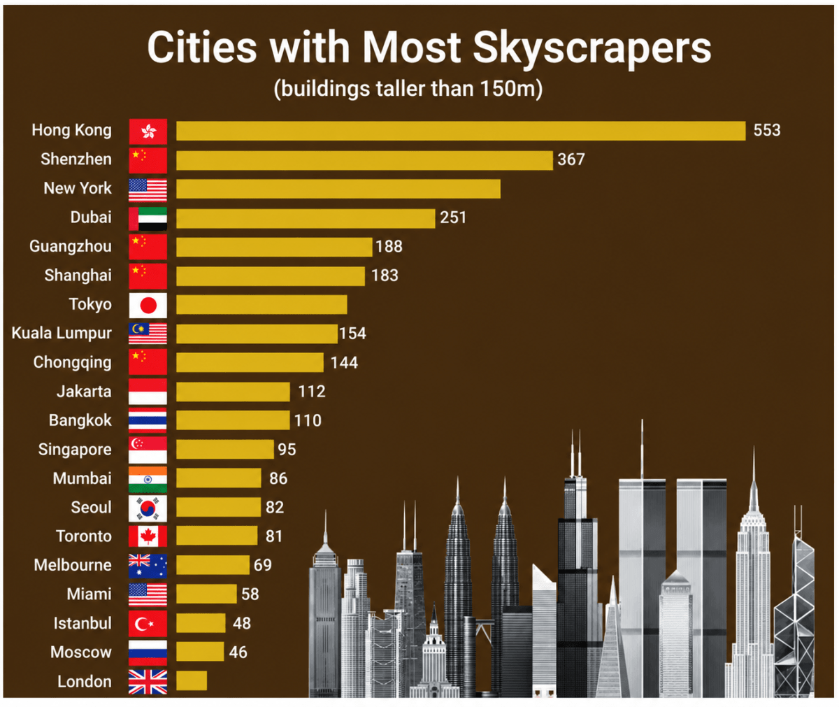
(a) Write estimated values for the number of skyscrapers in New York, Tokyo, and London.
(b) Are the following statements valid?
- Only 12 cities have more skyscrapers than Mumbai.
- Only 7 cities have fewer skyscrapers than Mumbai.
- The tallest building in the world is in Hong Kong.
Answer
The graph is titled 'Cities with Most Skyscrapers (buildings taller than 150 m)'. It lists 20 cities, arranged from the largest number of skyscrapers to the smallest:
Hong Kong 553, Shenzhen 367, New York —, Dubai 251, Guangzhou 188, Shanghai 183, Tokyo —, Kuala Lumpur 154, Chongqing 144, Jakarta 112, Bangkok 110, Singapore 95, Mumbai 86, Seoul 82, Toronto 81, Melbourne 69, Miami 58, Istanbul 48, Moscow 46, London —.
(a) The numbers for New York, Tokyo and London are not printed on the graph. So, we estimate them by comparing the lengths of their bars with the bars whose values are given.
The bar for New York is longer than the bar for Dubai (251) and shorter than the bar for Shenzhen (367), and lies nearly midway between the two. So, New York has about 310 skyscrapers.
The bar for Tokyo is shorter than the bar for Shanghai (183) and longer than the bar for Kuala Lumpur (154), and lies a little above the middle of the two. So, Tokyo has about 165 skyscrapers.
The bar for London is a little shorter than the bar for Moscow (46). So, London has about 40 skyscrapers.
Hence, New York has about 310 skyscrapers, Tokyo about 165 skyscrapers and London about 40 skyscrapers.
(b)
(i) Only 12 cities have more skyscrapers than Mumbai.
Mumbai is the 13th city in the graph.
Therefore, 12 cities are above Mumbai.
Hence, the statement is valid.
(ii) Only 7 cities have fewer skyscrapers than Mumbai.
The graph shows only 20 selected cities with the most skyscrapers. Although only seven cities shown have fewer skyscrapers than Mumbai, many other cities of the world are not included in this graph and may also have fewer skyscrapers.
Hence, the statement is not valid.
(iii) The tallest building in the world is in Hong Kong.
The graph gives the number of buildings taller than 150 m in each city. It does not tell us the height of the tallest building in any city.
Therefore, we cannot conclude that the tallest building in the world is in Hong Kong.
Hence, the statement is not valid.
Aditi likes solving puzzles. She recently started attempting the 'Easy' level Sudoku puzzles. The time she took (in seconds) to solve these puzzles are — 410, 400, 370, 340, 360, 400, 320, 330, 310, 320, 290, 380, 280, 270, 230, 220, 240. The first nine values correspond to Week 1 and the rest to Week 2.
(a) Construct a dot plot below showing the data for both weeks.
(b) Describe the mean, median, and any observations you may have about the data.

Answer
The data is:
Week 1: 410, 400, 370, 340, 360, 400, 320, 330, 310
Week 2: 320, 290, 380, 280, 270, 230, 220, 240
Draw the dot plot by marking the observations for Week 1 and Week 2 on the given scale.
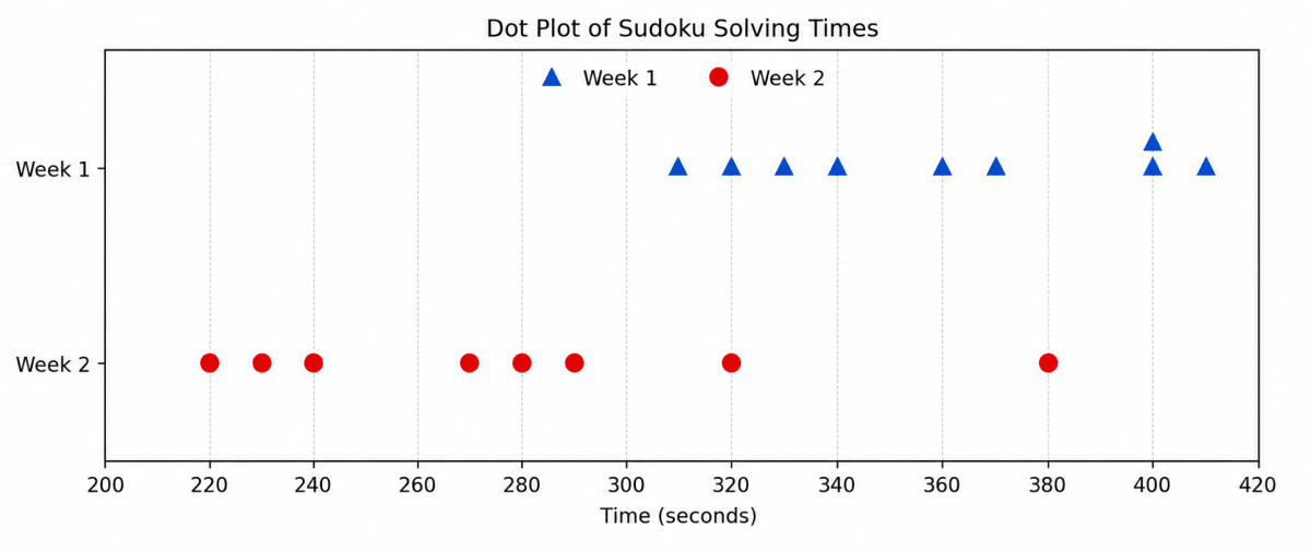
(b) Week 1
Sum of all observations = 410 + 400 + 370 + 340 + 360 + 400 + 320 + 330 + 310 = 3240
Number of all observations = 9
Mean time =
Arrange the data in ascending order:
310, 320, 330, 340, 360, 370, 400, 400, 410
There are 9 observations.
The middle (5th) observation is 360.
Median = 360 seconds
Week 2
Sum of all observations = 320 + 290 + 380 + 280 + 270 + 230 + 220 + 240 = 2230
Number of all observations = 8
Mean time =
Arrange the data in ascending order:
220, 230, 240, 270, 280, 290, 320, 380
There are 8 observations.
The two middle observations are 270 and 280.
Median =
Observations:
- The mean time decreases from 360 seconds in Week 1 to 278.75 seconds in Week 2.
- The median also decreases from 360 seconds to 275 seconds.
- This shows that Aditi solved the puzzles faster in Week 2 than in Week 1.
- In Week 1, the mean and median are equal, showing that the data is fairly balanced.
- In Week 2, the mean is slightly greater than the median because the value 380 seconds is much larger than the other times and pulls the mean upwards.
- The times in Week 2 are more spread out than those in Week 1.
Hence, the mean and median are both 360 seconds in Week 1, while in Week 2 the mean is 278.75 seconds and the median is 275 seconds. This shows that Aditi's speed improved in the second week.
Connect the Dots…
A number lock has a 3-digit code. Find the code using the hints below.
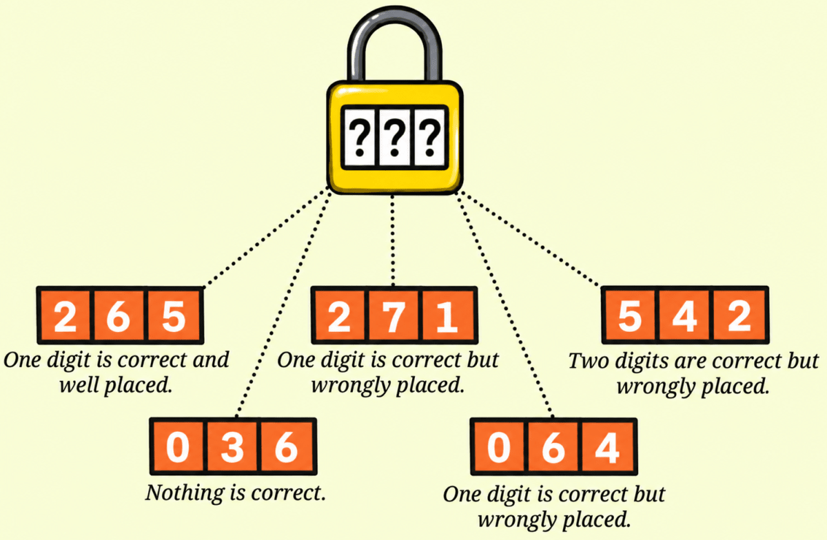
- 2 6 5 — One digit is correct and well placed.
- 2 7 1 — One digit is correct but wrongly placed.
- 5 4 2 — Two digits are correct but wrongly placed.
- 0 3 6 — Nothing is correct.
- 0 6 4 — One digit is correct but wrongly placed.
Answer
Let the three places of the code be called the first place, the second place and the third place.
Step 1: From the hint '0 3 6 — Nothing is correct', none of the digits 0, 3 and 6 is present in the code.
Step 2: Consider the hint '0 6 4 — One digit is correct but wrongly placed'. By Step 1, the digits 0 and 6 are not in the code. So, the one correct digit must be 4. As it is wrongly placed here, 4 is not in the third place. So, 4 is either in the first place or in the second place.
Step 3: Consider the hint '5 4 2 — Two digits are correct but wrongly placed'. Here 4 is again wrongly placed, so 4 is not in the second place either.
Combining Steps 2 and 3, we get that 4 is in the first place.
Step 4: Consider the hint '2 6 5 — One digit is correct and well placed'. By Step 1, the digit 6 is not in the code. So, exactly one of the digits 2 and 5 is in the code, and it is in the very place shown here.
If that digit were 2, then 2 would be in the first place. But by Step 3 the first place is taken by 4. So, that digit is not 2.
Therefore the correct digit is 5, and 5 is in the third place. Also, 2 is not present in the code.
Step 5: So far the code is 4 __ 5. Let us check this against the hint '5 4 2 — Two digits are correct but wrongly placed'. The two correct digits are 5 and 4 (as 2 is not in the code). In this hint 5 is in the first place while it actually belongs to the third place, and 4 is in the second place while it actually belongs to the first place. So, both are indeed wrongly placed, and the hint is satisfied.
Step 6: Consider the hint '2 7 1 — One digit is correct but wrongly placed'. By Step 4, the digit 2 is not in the code. So, exactly one of the digits 7 and 1 is in the code, and it must occupy the only place left — the second place.
If that digit were 7, then 7 would be in the second place. But in this hint 7 is already shown in the second place, so it would be well placed — which contradicts the hint.
Therefore the correct digit is 1, and 1 is in the second place.
So, the code is 4 1 5.
Verification: Let us check the code 415 against all the five hints.
| Hint | Check against the code 415 | Agrees? |
|---|---|---|
| 2 6 5 | 2 and 6 are absent; 5 is in the third place in both — one digit correct and well placed | Yes |
| 2 7 1 | 2 and 7 are absent; 1 is in the code but in the second place, not the third — one digit correct but wrongly placed | Yes |
| 5 4 2 | 2 is absent; 5 belongs to the third place, 4 belongs to the first place — two digits correct but wrongly placed | Yes |
| 0 3 6 | 0, 3 and 6 are all absent — nothing is correct | Yes |
| 0 6 4 | 0 and 6 are absent; 4 is in the code but in the first place, not the third — one digit correct but wrongly placed | Yes |
Hence, the 3-digit code of the number lock is 415.