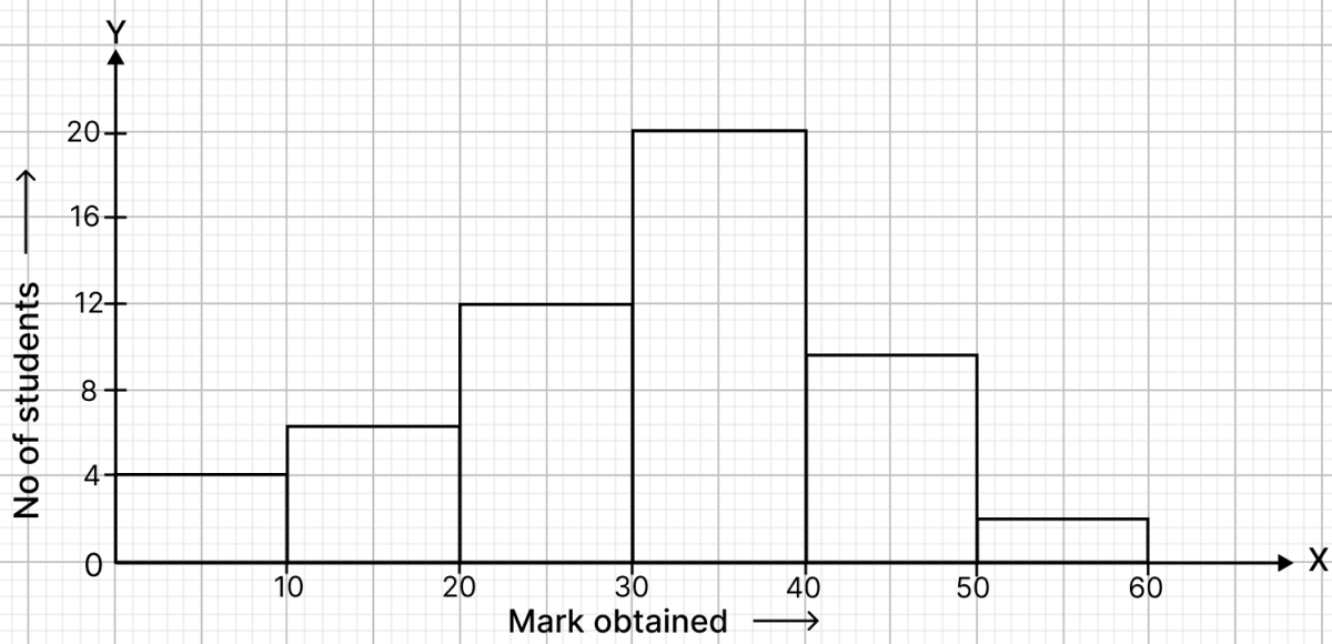
Draw a histogram to represent the following data :
| Marks obtained | No. of students |
|---|---|
| 0 - 10 | 4 |
| 10 - 20 | 7 |
| 20 - 30 | 12 |
| 30 - 40 | 20 |
| 40 - 50 | 9 |
| 50 - 60 | 2 |
Answer
Steps of construction of histogram :
Take 2 cm along x-axis = 10 units
Take 1 cm along y-axis = 4 units
Construct rectangles corresponding to the above continuous frequency distribution table.
The required histogram is shown in the below figure:
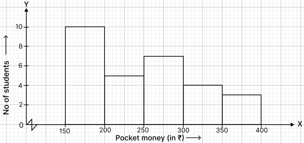
Draw a histogram to represent the following data :
| Pocket money (in ₹) | No. of students |
|---|---|
| 150 - 200 | 10 |
| 200 - 250 | 5 |
| 250 - 300 | 7 |
| 300 - 350 | 4 |
| 350 - 400 | 3 |
Answer
Steps of construction of histogram:
Since, the scale on x-axis starts at 150, a break (kink) is shown near the origin on x-axis to indicate that the graph is drawn to scale beginning at 150.
Take 2 cm along x-axis = 50 units.
Take 1 cm along y-axis = 2 units.
Construct rectangles corresponding to the above continuous frequency distribution table.
The required histogram is shown in the below figure :
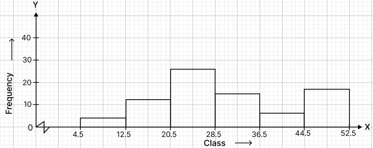
Construct a histogram for the following frequency distribution :
| Class interval | Frequency |
|---|---|
| 5 - 12 | 4 |
| 13 - 20 | 12 |
| 21 - 28 | 26 |
| 29 - 36 | 15 |
| 37 - 44 | 6 |
| 45 - 52 | 18 |
Answer
The above frequency distribution is discontinuous, to convert it into continuous frequency distribution,
Subtract the adjustment factor (0.5) from all the lower limits and add the adjustment factor (0.5) to all the upper limits.
Continuous frequency distribution for the given data is :
| CLasses before adjustment | Classes after adjustment | Frequency |
|---|---|---|
| 5 - 12 | 4.5 - 12.5 | 4 |
| 13 - 20 | 12.5 - 20.5 | 12 |
| 21 - 28 | 20.5 - 28.5 | 26 |
| 29 - 36 | 28.5 - 36.5 | 15 |
| 37 - 44 | 36.5 - 44.5 | 6 |
| 45 - 52 | 44.5 - 52.5 | 18 |
Steps of construction :
Take 2 cm along x-axis = 8 units.
Take 1 cm along y-axis = 10 units.
A kink is drawn near x-axis to show that the scale starts from 4.5 and not zero.
Construct rectangles corresponding to the above continuous frequency distribution table.
The required histogram is shown in the below figure:
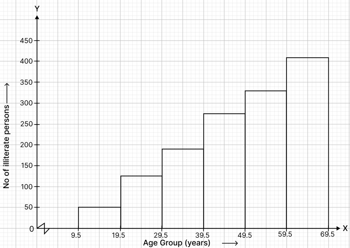
The following table shows the number of illiterate persons in the age group (10 - 69) in a town
| Age group (in years) | No. of illiterate persons |
|---|---|
| 10 - 19 | 50 |
| 20 - 29 | 125 |
| 30 - 39 | 190 |
| 40 - 49 | 275 |
| 50 - 59 | 340 |
| 60 - 69 | 410 |
Draw a histogram to represent the above data.
Answer
The following frequency distribution is discontinuous, to convert it into continuous frequency distribution,
Subtract the adjustment factor (0.5) from all the lower limits and add the adjustment factor (0.5) to all the upper limits.
Continuous frequency distribution for the given data is :
| Age group before adjustment | Age group after adjustment | No. of illiterate persons (Frequency) |
|---|---|---|
| 10 - 19 | 9.5 - 19.5 | 50 |
| 20 - 29 | 19.5 - 29.5 | 125 |
| 30 - 39 | 29.5 - 39.5 | 190 |
| 40 - 49 | 39.5 - 49.5 | 275 |
| 50 - 59 | 49.5 - 59.5 | 340 |
| 60 - 69 | 59.5 - 69.5 | 410 |
Steps of construction :
Take 2 cm along x-axis = 10 years
Take 1 cm along y-axis = 50 units
A kink is drawn near x-axis to show that the scale starts from 9.5 and not zero.
Construct rectangles corresponding to the above continuous frequency distribution table.
The required histogram is shown in the below figure:
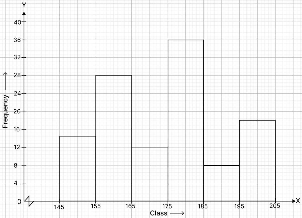
Draw a histogram to represent the following data :
| Class mark | Frequency |
|---|---|
| 150 | 15 |
| 160 | 28 |
| 170 | 12 |
| 180 | 36 |
| 190 | 8 |
| 200 | 18 |
Draw a histogram to represent the above data.
Answer
Since, the difference between the values of any two consecutive class marks is 10 (160 - 150)
∴ subtract = 5, from each class mark to get the lower limit of the corresponding class interval and add 5 to each class mark to get the upper limit.
Frequency distribution table :
| Class mark | Class | Frequency |
|---|---|---|
| 150 | 145 - 155 | 15 |
| 160 | 155 - 165 | 28 |
| 170 | 165 - 175 | 12 |
| 180 | 175 - 185 | 36 |
| 190 | 185 - 195 | 8 |
| 200 | 195 - 205 | 18 |
Steps of construction of histogram :
Since, the scale on x-axis starts at 145, a break (kink) is shown near the origin on x-axis to indicate that the graph is drawn to scale beginning at 145.
Take 2 cm along x-axis = 10 units.
Take 1 cm along y-axis = 4 units.
Construct rectangles corresponding to the above continuous frequency distribution table.
The required histogram is shown in the below figure :
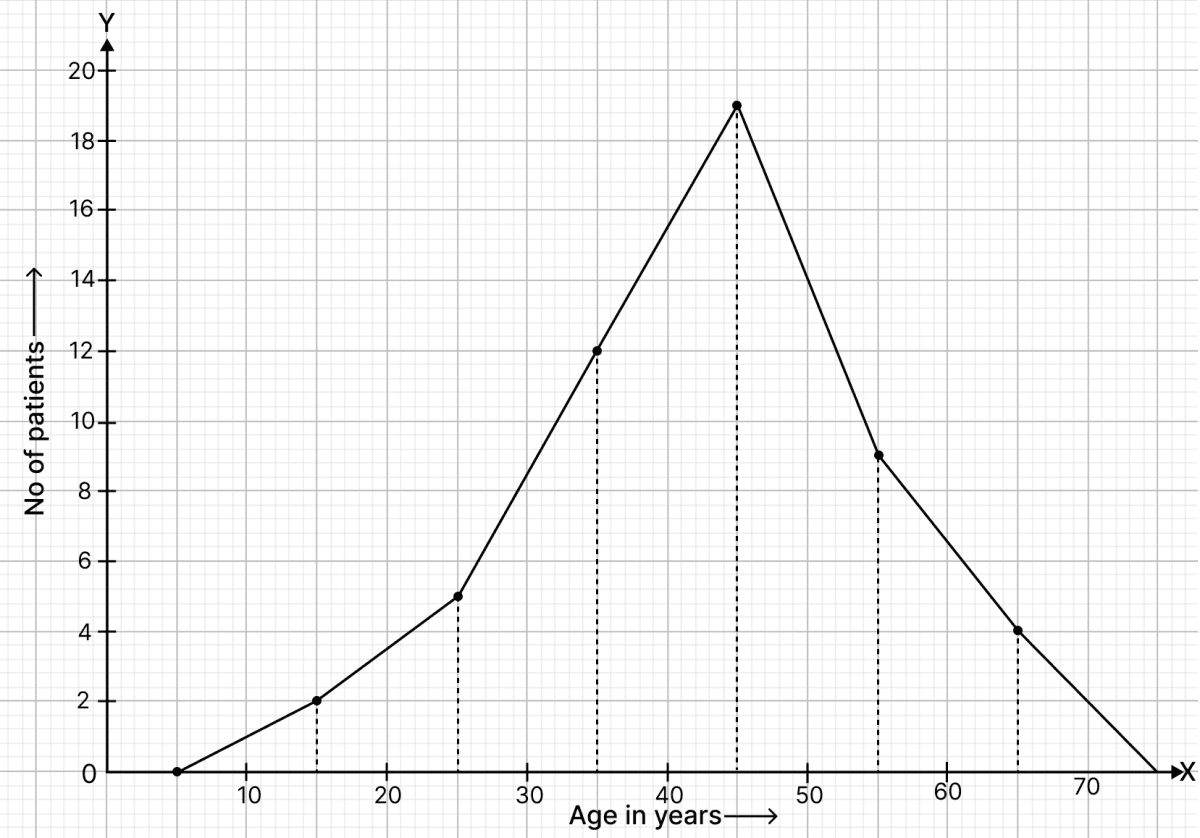
In a study of diabetic patients in a village, the following observations were noted :
| Age in years | No. of patients |
|---|---|
| 10 - 20 | 2 |
| 20 - 30 | 5 |
| 30 - 40 | 12 |
| 40 - 50 | 19 |
| 50 - 60 | 9 |
| 60 - 70 | 4 |
Represent the above data by a frequency polygon.
Answer
Frequency distribution table :
| Age in years | Class marks | No. of patients |
|---|---|---|
| 10 - 20 | 15 | 2 |
| 20 - 30 | 25 | 5 |
| 30 - 40 | 35 | 12 |
| 40 - 50 | 45 | 19 |
| 50 - 60 | 55 | 9 |
| 60 - 70 | 65 | 4 |
Steps of construction of frequency polygon:
Take 2 cm along x-axis = 10 years.
Take 1 cm along y-axis = 2 patients.
Find the mid-points of class intervals.
Find points corresponding to given frequencies of classes and the mid-points of class intervals, and plot them.
Join consecutive points by line segments.
Join first end point with mid-point of class 0 - 10 with zero frequency and join the other end with mid point of class 70 - 80 with zero frequency.
The required frequency polygon is shown alongside.
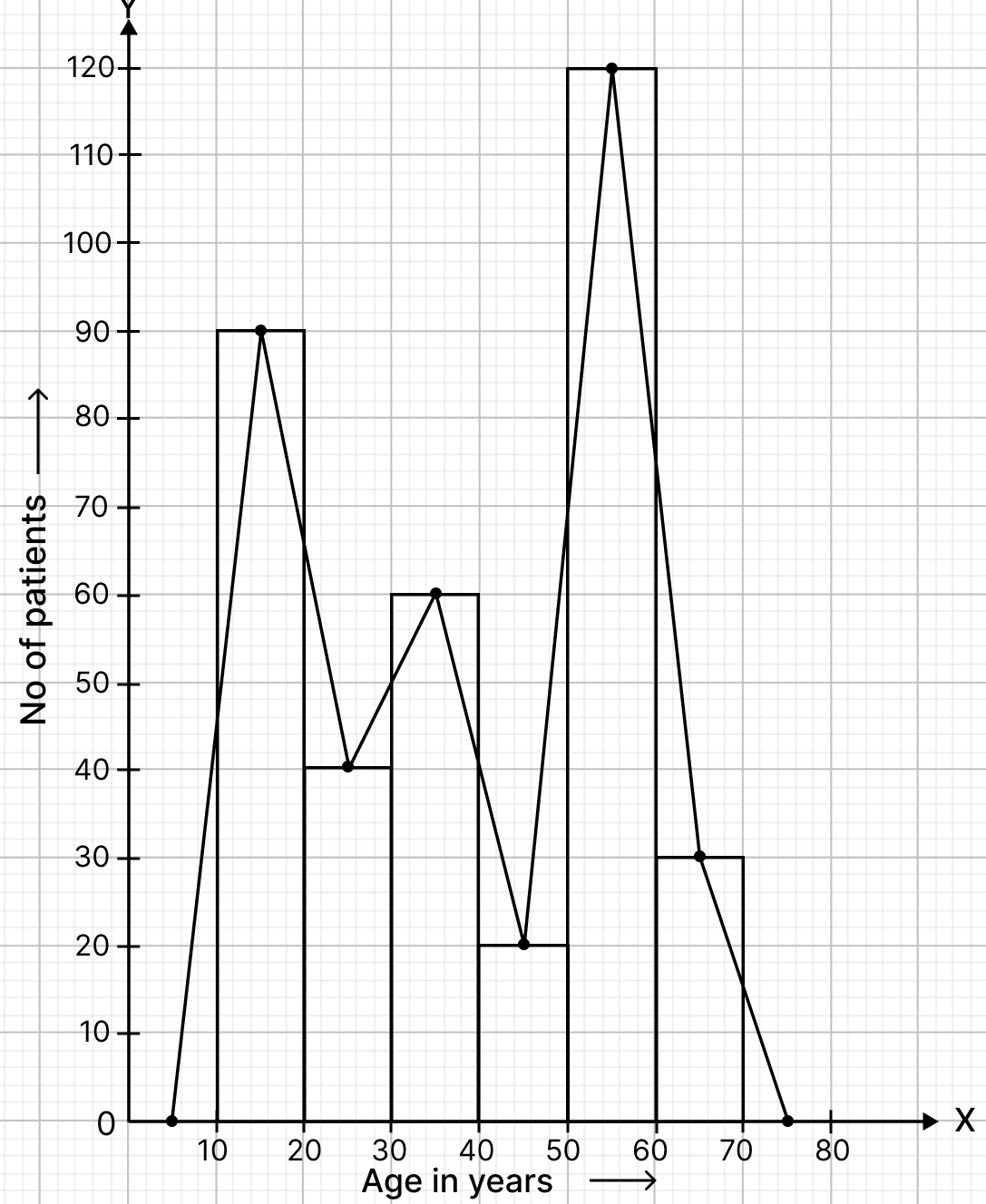
The ages (in years) of 360 patients treated in a hospital on a particular day are given below :
| Age in years | No. of patients |
|---|---|
| 10 - 20 | 90 |
| 20 - 30 | 40 |
| 30 - 40 | 60 |
| 40 - 50 | 20 |
| 50 - 60 | 120 |
| 60 - 70 | 30 |
Draw a histogram and a frequency polygon on the same graph to represent the above data.
Answer
Frequency distribution table :
| Age in years | Class marks | No. of patients |
|---|---|---|
| 10 - 20 | 15 | 90 |
| 20 - 30 | 25 | 40 |
| 30 - 40 | 35 | 60 |
| 40 - 50 | 45 | 20 |
| 50 - 60 | 55 | 120 |
| 60 - 70 | 65 | 30 |
Steps of construction of histogram :
Take 1 cm along x-axis = 10 years.
Take 1 cm along y-axis = 10 patients.
Construct rectangles corresponding to the above continuous frequency distribution table.
Steps of construction of frequency polygon:
Mark the mid-points of upper bases of rectangles of the histogram.
Join the consecutive mid-points by line-segments.
Join first end point with mid-point of class 0 - 10 with zero frequency, and join the other end point with the mid point of class 70 - 80 with zero frequency.
The required frequency polygon is shown by thick line segments in the diagram.
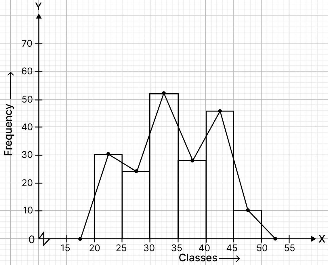
Draw a histogram and the frequency polygon from the following data:
| Class interval | Frequency |
|---|---|
| 20 - 25 | 30 |
| 25 - 30 | 24 |
| 30 - 35 | 52 |
| 35 - 40 | 28 |
| 40 - 45 | 46 |
| 45 - 50 | 10 |
Answer
Frequency distribution table :
| Class interval | Class marks | Frequency |
|---|---|---|
| 20 - 25 | 22.5 | 30 |
| 25 - 30 | 27.5 | 24 |
| 30 - 35 | 32.5 | 52 |
| 35 - 40 | 37.5 | 28 |
| 40 - 45 | 42.5 | 46 |
| 45 - 50 | 47.5 | 10 |
Steps of construction of histogram:
Since, the scale on x-axis starts at 15, a break (kink) is shown near the origin on x-axis to indicate that the graph is drawn to scale beginning at 15.
Take 1 cm along x-axis = 5 units.
Take 1 cm along y-axis = 10 units.
Construct rectangles corresponding to the above continuous frequency distribution table.
Steps of construction of frequency polygon:
Mark the mid-points of upper bases of rectangles of the histogram.
Join the consecutive mid-points by line-segments.
Join first end point with mid-point of class 15 - 20 with zero frequency, and join the other end point with the mid point of class 50 - 55 with zero frequency.
The required frequency polygon is shown by thick line segments in the diagram.
Draw a histogram for the following data:
| Class interval | Frequency |
|---|---|
| 600 - 640 | 18 |
| 640 - 680 | 45 |
| 680 - 720 | 153 |
| 720 - 760 | 288 |
| 760 - 800 | 171 |
| 800 - 840 | 63 |
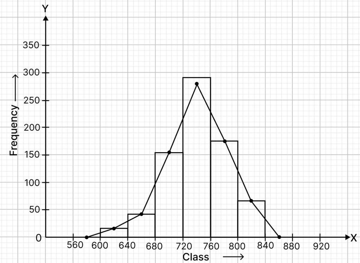
Using this histogram, draw the frequency polygon on the same graph.
Answer
Frequency distribution table :
| Class interval | Class marks | Frequency |
|---|---|---|
| 600 - 640 | 620 | 18 |
| 640 - 680 | 660 | 45 |
| 680 - 720 | 700 | 153 |
| 720 - 760 | 740 | 288 |
| 760 - 800 | 780 | 171 |
| 800 - 840 | 820 | 63 |
Steps of construction of histogram:
Since, the scale on x-axis starts at 560, a break (kink) is shown near the origin on x-axis to indicate that the graph is drawn to scale beginning at 560.
Take 1 cm along x-axis = 40 units.
Take 1 cm along y-axis = 50 units.
Construct rectangles corresponding to the above continuous frequency distribution table.
Steps of construction of frequency polygon:
Mark the mid-points of upper bases of rectangles of the histogram.
Join the consecutive mid-points by line-segments.
Join first end point with mid-point of class (560 - 600) with zero frequency, and join the other end point with the mid point of class (840 - 880) with zero frequency.
The required frequency polygon is shown by thick line segments in the diagram.
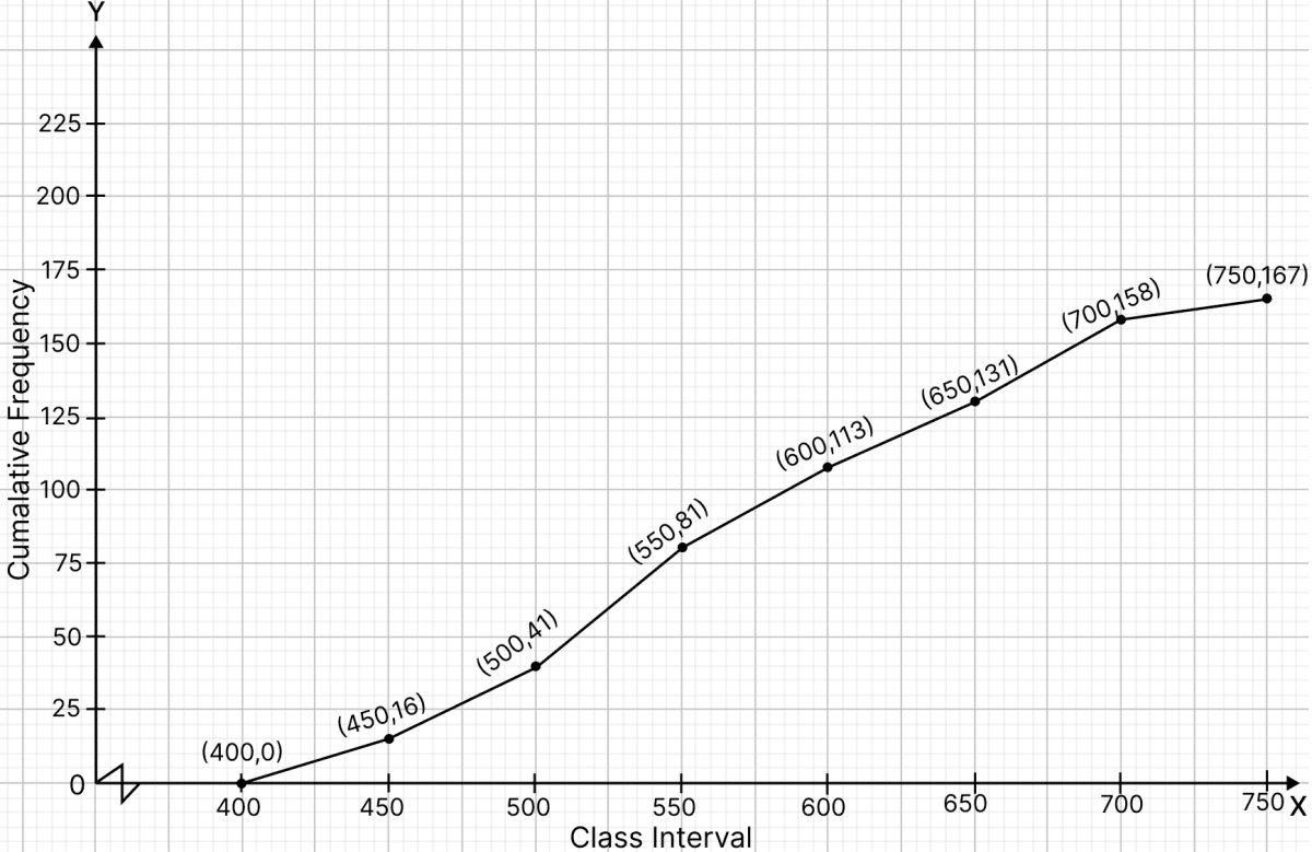
Draw an ogive to represent the following data:
| Class interval | Frequency |
|---|---|
| 400 - 450 | 16 |
| 450 - 500 | 25 |
| 500 - 550 | 40 |
| 550 - 600 | 32 |
| 600 - 650 | 18 |
| 650 - 700 | 27 |
| 700 - 750 | 9 |
Answer
The cumulative frequency distribution :
| Class interval | Frequency | Cumulative frequency |
|---|---|---|
| 400 - 450 | 16 | 16 |
| 450 - 500 | 25 | 41 (16 + 25) |
| 500 - 550 | 40 | 81 (41 + 40) |
| 550 - 600 | 32 | 113 (81 + 32) |
| 600 - 650 | 18 | 131 (113 + 18) |
| 650 - 700 | 27 | 158 (131 + 27) |
| 700 - 750 | 9 | 167 (158 + 9) |
Steps of construction of ogive:
Take 2 cm = 50 units along x-axis.
Take 1 cm = 25 units along y-axis.
Ogive always starts from a point on x-axis representing the lower limit of the first class. Mark point (400, 0).
Take upper class limits along x-axis and corresponding cumulative frequencies along y-axis, mark the points (450, 16), (500, 41), (550, 81), (600, 113), (650, 131), (700, 158) and (750, 167).
Join the points marked by a free hand curve.
The required ogive is shown in the below figure:
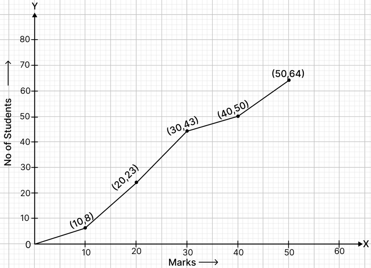
Draw an ogive for the following frequency distribution:
| Marks obtained | No. of students |
|---|---|
| Less than 10 | 8 |
| Less than 20 | 23 |
| Less than 30 | 43 |
| Less than 40 | 50 |
| Less than 50 | 64 |
Answer
The cumulative frequency distribution :
| Marks obtained | Class interval | No. of students (Cumulative frequency) |
|---|---|---|
| Less than 10 | 0 - 10 | 8 |
| Less than 20 | 10 - 20 | 23 |
| Less than 30 | 20 - 30 | 43 |
| Less than 40 | 30 - 40 | 50 |
| Less than 50 | 40 - 50 | 64 |
Steps of construction of ogive:
Take 2 cm = 10 marks along x-axis.
Take 1 cm = 10 students along y-axis.
Ogive always starts from a point on x-axis representing the lower limit of the first class. Mark point (0, 0).
Take upper class limits along x-axis and corresponding cumulative frequencies along y-axis, mark the points (10, 8), (20, 23), (30, 43), (40, 50), (50, 64).
Join the points marked by a free hand curve.
The required ogive is shown in the below figure:
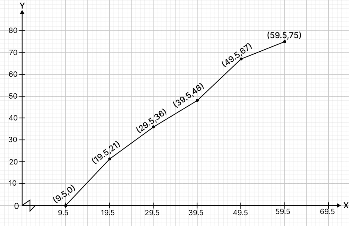
Draw an ogive for the following frequency distribution :
| Class - interval | Frequency |
|---|---|
| 10 - 19 | 21 |
| 20 - 29 | 15 |
| 30 - 39 | 12 |
| 40 - 49 | 19 |
| 50 - 59 | 8 |
Answer
The above frequency distribution is discontinuous, to convert it into continuous frequency distribution,
Subtract the adjustment factor (0.5) from all the lower limits and add the adjustment factor (0.5) to all the upper limits.
Continuous frequency distribution for the given data is :
| Classes before adjustment | Classes after adjustment | Frequency | Cumulative frequency |
|---|---|---|---|
| 10 - 19 | 9.5 - 19.5 | 21 | 21 |
| 20 - 29 | 19.5 - 29.5 | 15 | 36 (21 + 15) |
| 30 - 39 | 29.5 - 39.5 | 12 | 48 (36 + 12) |
| 40 - 49 | 39.5 - 49.5 | 19 | 67 (48 + 19) |
| 50 - 59 | 49.5 - 59.5 | 8 | 75 (67 + 8) |
Steps of construction :
Since, the scale on x-axis starts at 9.5, a break (kink) is shown near the origin on x-axis to indicate that the graph is drawn to scale beginning at 9.5.
Take 2 cm along x-axis = 10 units
Take 1 cm along y-axis = 10 units
Ogive always starts from a point on x-axis representing the lower limit of the first class. Mark point (9.5, 0).
Take upper class limits along x-axis and corresponding cumulative frequencies along y-axis, mark the points (19.5, 21), (29.5, 36), (39.5, 48), (49.5, 67), (59.5, 75).
Join the points marked by a free hand curve.
The required ogive is shown in the below figure:
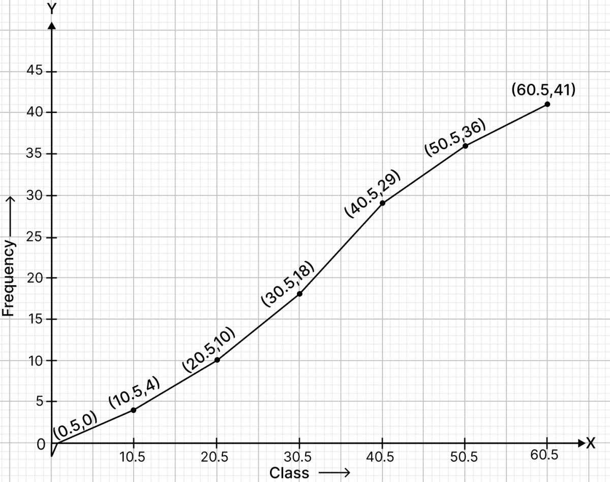
Draw an ogive for the following data:
| Class - interval | Frequency |
|---|---|
| 1 - 10 | 4 |
| 11 - 20 | 6 |
| 21 - 30 | 8 |
| 31 - 40 | 11 |
| 41 - 50 | 7 |
| 51 - 60 | 5 |
Answer
The above frequency distribution is discontinuous, to convert it into continuous frequency distribution,
Subtract the adjustment factor (0.5) from all the lower limits and add the adjustment factor (0.5) to all the upper limits.
Continuous frequency distribution for the given data is :
| CLasses before adjustment | Classes after adjustment | Frequency | Cumulative frequency |
|---|---|---|---|
| 1 - 10 | 0.5 - 10.5 | 4 | 4 |
| 11 - 20 | 10.5 - 20.5 | 6 | 10 (6 + 4) |
| 21 - 30 | 20.5 - 30.5 | 8 | 18 (10 + 8) |
| 31 - 40 | 30.5 - 40.5 | 11 | 29 (18 + 11) |
| 41 - 50 | 40.5 - 50.5 | 7 | 36 (29 + 7) |
| 51 - 60 | 50.5 - 60.5 | 5 | 41 (36 + 5) |
Steps of construction :
Since, the scale on x-axis starts at 10.5, a break (kink) is shown near the origin on x-axis to indicate that the graph is drawn to scale beginning at 10.5.
Take 2 cm along x-axis = 10 units
Take 1 cm along y-axis = 5 units
Ogive always starts from a point on x-axis representing the lower limit of the first class. Mark point (0.5, 0).
Take upper class limits along x-axis and corresponding cumulative frequencies along y-axis, mark the points (10.5, 4), (20.5, 10), (30.5, 18), (40.5, 29), (50.5, 36), (60.5, 41).
Join the points marked by a free hand curve.
The required ogive is shown in the below figure: