
In OOo Calc formula starts with ............... .
- +
- [= sign]
- -
- *
Answer
[= sign]
Reason — In OOo Calc formula starts with equal to ( = ) sign.
The cell having bold boundary is the ............... cell.
- Last
- Next
- First
- Active
Answer
Active
Reason — The cell having bold boundary is the active cell.
In ............... referencing the relative address of the cell gets adjusted w.r.t. the current cell.
- Relative
- Absolute
- Mixed
- Nil
Answer
Relative
Reason — In relative referencing the relative address of the cell gets adjusted w.r.t. the current cell.
To create an absolute cell reference ............... sign is used before the parts of formula.
- $ sign
- #
- ^
- %
Answer
$ sign
Reason — To create an absolute cell reference $ sign is used before the parts of formula.
Calc worksheets are given ............... extension.
- .odf
- [= sign]
- .ods
- .odw
Answer
.ods
Reason — Calc worksheets are given .ods extension.
Cell address A4 in a formula means it is a :
- Mixed cell reference
- Absolute cell reference
- Relative cell reference
- None of the above
Answer
Relative cell reference
Reason — Cell address A4 in a formula means it is a Relative cell reference as in this cell referencing technique, the cells are referred to by their relative position in the worksheet.
Cell address $A$4 in a formula means it is a :
- Mixed cell reference
- Absolute cell reference
- Relative cell reference
- All the above.
Answer
Absolute cell reference
Reason — Cell address $A$4 in a formula means it is an Absolute cell reference because the use of $ sign makes the column and row absolute, i.e., the address will not change when the formula is copied to any other cell.
Cell address $A4 in a formula means it is a :
- Mixed cell reference
- Absolute cell reference
- Relative cell reference
- All the above.
Answer
Mixed cell reference
Reason — Cell address $A4 in a formula means it is a Mixed cell reference because the column A is absolute while the row 4 is relative. Thus, when the formula is copied to any other location, the column will remain the same while the row will change.
Cell address A$4 in a formula means it is a :
- Mixed cell reference
- Absolute cell reference
- Relative cell reference
- None of the above
Answer
Mixed cell reference
Reason — Cell address A$4 in a formula means it is a Mixed cell reference because the column A is relative while the row 4 is absolute. Thus, when the formula is copied to any other location, the column will change while the row will remain the same.
How would you refer to the range starting from 1st column, 1st row and spread till 6th column and 3rd row ?
- [E3 : A1]
- [A1 : E3]
- [I6 : A1]
- [A1 : F3]
Answer
[A1 : F3]
Reason — The cell address of 1st column, 1st row is A1 and the cell address of 6th column and 3rd row is F3. Since a range is specified by giving the addresses of the first cell and the last cell in the range, the range will be referred as [A1 : F3].
The keyboard shortcut for Copy is ................ and for Paste is ................. .
- Ctrl + C
- Ctrl + X
- Ctrl + A
- Ctrl + V
Answer
Ctrl + C, Ctrl + V
Reason — The keyboard shortcut for Copy is Ctrl + C and for Paste is Ctrl + V.
When you ................. or ................. , the selected range gets surrounded by a moving border.
- Copy, Paste
- Copy
- Cut
- Cut, Paste
Answer
Copy, Cut
Reason — When you copy or cut, the selected range gets surrounded by a moving border.
The ............... operation copies data from the source range to target range and erases it from the source range.
- Cut and Copy
- Cut, Copy and Paste
- Copy and Paste
- Cut and Paste
Answer
Cut and Paste
Reason — The Cut and Paste operation copies data from the source range to target range and erases it from the source range.
If you enter 12 + 24 in a cell, Calc will display ...............
- 36
- A12 + A24
- A12 : A24
- 12 + 24
Answer
12 + 24
Reason — If we enter 12 + 24 in a cell, Calc will treat it as text and display it as it is i.e., 12 + 24 and not 36.
Address of the cell at 20th column and 30th row is ............... .
- T20
- T30
- 20, 30
- 30T
Answer
T30
Reason — Address of the cell at 20th column and 30th row is T30 because this cell is formed by the intersection of column T and row 30.
The formula in cell A2 is = B2 + C3. On copying this formula to cell C2, the formula in cell C2 will be ................. .
- = B2 + C3
- = C3 + B2
- = D2 + E3
- = E3 + D2
Answer
= D2 + E3
Reason — When we copy the formula from cell A2 to cell C2, Calc adjusts the relative cell references in the formula based on the new location. When we copy the original formula "= B2 + C3" to cell C2, Calc will adjust the formula to "= D2 + E3", where it shifts the column references by 2 columns to the right and keeps the row references the same.
Cancel button (x on formula bar) can be used to undo a cell entry after it has been completed.
- True
- False
Answer
True
Reason — Cancel button (x on formula bar) can be used to undo a cell entry after it has been completed.
All formulas start with an = sign in Calc.
- True
- False
Answer
True
Reason — All formulas start with an = sign in Calc.
If you enter 127A in a cell it will be treated as a number because it starts with a digit.
- True
- False
Answer
False
Reason — Any combination of numbers, spaces and non-numeric characters (such as 127A) is treated as text.
A cell entry can be edited either in the cell or in the formula bar.
- True
- False
Answer
True
Reason — A cell entry can be edited either in the cell or in the formula bar.
When you clear only the contents of a cell, all the formats and contents are deleted.
- True
- False
Answer
False
Reason — When we clear only the contents of a cell, the formats and comments remain intact and only the contents of the cell are deleted.
You cannot open two different workbooks in Calc simultaneously.
- True
- False
Answer
False
Reason — We can open two different workbooks in Calc simultaneously.
When a cell containing a formula is moved, the cells referring the moved cell, show an error value.
- True
- False
Answer
False
Reason — When a cell containing a formula is moved, Calc automatically adjusts the references in the formula to reflect the new location of the cell. This adjustment is done to ensure that the formula still references the correct cells and data.
Once you copy data on to the clipboard, it can be copied to multiple ranges even after pressing Enter key.
- True
- False
Answer
False
Reason — After pasting data from clipboard into a range, the data won't automatically continue to be pasted into additional ranges after pressing Enter.
What is a cell and how is it referred in OOo Calc ?
Answer
Cell is a basic unit of worksheet where numbers, text, formulas etc. can be placed. Cell is formed by intersection of a row and a column, which gives a cell a unique address.
For instance, if row 3 is intersected by column F, then the cell formed out of it gets an address F3. Similarly, C5 identifies the cell in column C, row 5.
What do you mean by a range of cells ?
Answer
A range of cells is a group of contiguous cells that forms a rectangular area in shape.
A range is specified by giving the addresses of first cell and the last cell of the range. For instance, a range starting from F7 till G14 would be written as F7 : G14 in OOo Calc.
What is the difference between a worksheet and a workbook ?
Answer
| Worksheet | Workbook |
|---|---|
| A Worksheet is a grid of cells made up of rows and columns. | Multiple worksheets can be combined under a file known as Workbook. |
What are the different types of data that can be entered in OOo Calc.
Answer
The different types of data that can be entered in OOo Calc are:
- Numbers — These are numeric entries like 4362, 763.368 etc.
- Text — Text is any combination of numbers, spaces, and non-numeric characters like 43A, 123XYZ etc.
- Formulas — Formula is a sequence of values, cell-addresses, names, functions or operators in a cell that produces a new value from existing values. For example, =A1+A2.
The keyboard shortcut for Copy is ................. and for Paste is ................. .
Answer
The keyboard shortcut for Copy is Ctrl + C and for Paste is Ctrl + V .
What will happen to the contents of the destination cell if you copy the contents of the source cell into the destination cell ?
Answer
If we copy the contents of the source cell and paste them into the destination cell, the contents of the destination cell will be replaced by the contents of the source cell. The original contents of the destination cell will be overwritten with the copied data from the source cell.
What is the name of the package which permits people to quickly create, manipulate and analyze data arranged in rows and columns ?
- Spreadsheet package
- Word processing package
- Outline processors
- Application package
Answer
Spreadsheet package
Reason — A spreadsheet package permits people to quickly create, manipulate and analyze data arranged in rows and columns.
What does an electronic spreadsheet consist of ?
- Rows
- Columns
- Cells
- All the above
Answer
All the above
Reaosn — An electronic spreadsheet consists of a grid of cells made up of horizontal rows and vertical columns.
State whether the following statements are true or false :
(i) When you increase the font size, the row height is automatically adjusted.
(ii) By default, the numbers are left aligned and text values are right aligned.
Answer
(i) True.
Reason — When we increase the font size, the row height is automatically adjusted.
(ii) False.
Reason — By default, the numbers are right aligned and text values are left aligned.
Write cell references for the following :
(i) Cell formed by intersection of row 18, and column Z.
(ii) The right most cell in row 32 in a worksheet.
(iii) If you select an entire worksheet, which range of cells gets selected.
(iv) Reference (Fixed Column and Relative row) formed by row 134 and column BD.
(v) Mixed Reference (Relative column and Fixed row) formed by row 120 and column IA
(vi) Absolute Reference formed by 45 and column Z.
(vii) Relative Reference formed by row 19 and column AB.
Answer
(i) Z18
(ii) ZZ32 (If ZZ is the last column)
(iii) All the cells get selected.
(iv) $BD134
(v) IA$120
(vi) $Z$45
(vii) AB19
Suggest the Calc functions that can be used for carrying out following operations :
(i) To calculate total marks of a student if his marks in five subjects are given in five different cells.
(ii) To calculate average sales made by salesman of a company, if sales made by each of the salesmen is available.
(iii) To find out the marks of top scorer in a class, if marks of all the students are available.
(iv) To find out minimum quoted rate from various quotations available.
Answer
(i) SUM
(ii) AVERAGE
(iii) MAX
(iv) MIN
What are the rules to be followed while entering the following in OOo Calc ?
(i) numbers
(ii) text
(iii) formulas
Answer
The rules to be followed while entering the following in OOo Calc are as follows:
(i) Numbers — A number can contain only the following characters :
0 1 2 3 4 5 6 7 8 9 + - ( ) , / $ % . E e
(ii) Text — Text is any combination of numbers, spaces, and non-numeric characters.
(iii) Formulas — A formula begins with an '=' sign and can contain values (entries that can be used for calculations), operators (e.g., +, /, *) and cell addresses (e.g., C9, B14).
Explain what are the different methods of cell referencing in OOo Calc ?
Answer
Cell referencing in OOo Calc are of three types :
- Relative referencing — Cell referencing in which the cells are referred by their relative position in the worksheet — relative to a particular cell is known as Relative referencing. For example, A23, BZ15 etc.
- Absolute referencing — Cell referencing in which the cells are referred by their fixed position (absolute position) in the worksheet is known as Absolute referencing. For example, $A$23, $Z$15 etc.
- Mixed Referencing — Combination of relative and absolute referencing is called mixed referencing. For example, A$23, $Z15 etc.
Differentiate between mixed referencing and absolute referencing by giving suitable examples.
Answer
| Mixed referencing | Absolute referencing |
|---|---|
| Mixed referencing fixes either the row or column while allowing the other to change. | In absolute referencing, both the row and column references are fixed. |
| When a formula with mixed references is copied to another cell, the absolute part of the reference remains fixed while the relative part of the reference changes. | When a formula with absolute references is copied to another cell, the references remain unchanged. |
| For example, C$6 is a mixed reference where column is relative and row is absolute. $C6 is also a mixed reference but here column is absolute and row is relative. | For example, $C$6 is an absolute reference where both row and column are fixed. |
What is the difference between copying and moving a range ?
Answer
| Copying a Range | Moving a Range |
|---|---|
| When we copy a range of cells, we create a duplicate copy of the selected cells. | When we move a range of cells, we are relocating the selected cells from their original location to a new location. |
| The original cells remain at their original location, and a copy is placed elsewhere in the worksheet. | The original cells are deleted from their original position and placed at the new location. |
| This is useful when we want to preserve the original data while using a copy for calculations, analysis, or other purposes. | This is useful when we want to reorganize our data within the same worksheet or between worksheets. |
What is the difference between the following commands :
Edit → Delete Contents → Delete all and
Edit → Delete Contents → TextEdit → Delete Contents → Text and
Edit → Delete Contents → FormatsEdit → Delete Contents → Text and
Edit → Delete Contents → Notes
Answer
The Delete All option deletes all content from the selected cell range.
The Text option deletes text only. Formats, formulas, numbers and dates are not affected.The Text option deletes text only and does not affect formats, formulas, numbers and dates.
The Formats option deletes format attributes applied to cells. All the cell content remains unchanged.The Text option deletes text only and does not affect formats, formulas, numbers and dates.
The Notes option deletes notes added to cells. All other elements remain unchanged.
Create the following worksheet and save the workbook as WAGES.ods.

(i) Find out the number of days each worker has worked, by subtracting date on which worker was hired from today's date.
(ii) Calculate Gross wages for each worker. The gross wages can be calculated by using the following formula :
Gross wages = No. of days worked * Pay rate
Answer
(i) To find out the number of days each worker has worked, follow the given steps:
Step 1 — Select cell C7 and type the formula =$C$3 - B7. Press Enter key. The number of working days will appear in the cell.
The given formula subtracts the date on which the worker was hired from today's date. This gives us the number of days the worker has worked.
Step 2 — With C7 selected, dragging the cell handle from C8 to C12 will copy the formula to the cell range [C8 : C12].
Notice that the formula =$C$3 - B7 will modify itself according to the cell. Cell address $C$3 is an absolute address, so it will not change. But the relative address B7 will change according to the position of the cell.
So, the formula =$C$3 - B8 will be pasted in cell C8, =$C$3 - B9 will be pasted in C9, =$C$3 - B10 will be pasted in cell C10 and so on.

(ii) To calculate the gross wages for each worker, follow the given steps:
Step 1 — Select cell D7 and type the formula =C7*$C$4. Press Enter key. The gross wages of Kushagra will appear in the cell.
The given formula multiplies the number of working days and the pay rate per day.
Step 2 — With D7 selected, dragging the cell handle from D8 to D12 will copy the formula to the cell range [D8 : D12].
Notice that the formula =C7*$C$4 will modify itself according to the cell. Cell address $C$4 is an absolute address, so it will not change. But the relative address C7 will change according to the position of the cell.
So, the formula =C8*$C$4 will be pasted in cell D8, =C9*$C$4 will be pasted in D9, =C10*$C$4 will be pasted in cell D10 and so on.

Create the following worksheet in Ooo Calc.
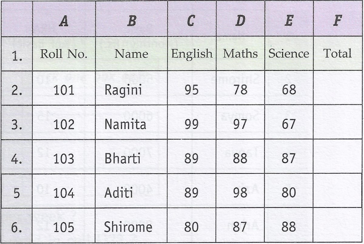
(i) From the above worksheet find out the average marks for the entire class.
(ii) Now copy the range consisting of the mentioned data (including total, average & class average) to a new location. Find out whether the cell references change or not.
(iii) Now move the original data range to a new location. Find out whether the cell references change or not.
(iv) Again move back the data to its original position and make changes in the marks obtained by students. Notice total, average and class average. What happens ? Why does this happen ?
Answer
(i) The average marks for the entire class is 86.

We follow the following steps to find the average marks for the entire class:
Step 1 — Find the total marks for each student.
Select F2 and write the formula =SUM(C2:E2). This formula will calculate the total marks of a student.
With F2 selected, dragging the cell handle from F3 to F6 will copy the formula to the cell range [F3 : F6].
Step 2 — Find the average marks for each student.
Select G2 and write the formula =AVERAGE(C2:E2). This formula will calculate the average marks of a student.
With G2 selected, dragging the cell handle from G3 to G6 will copy the formula to the cell range [G3 : G6].
Step 3 — Find the average marks for the entire class.
Select cell G7 and write the formula =AVERAGE(G2 : G6).
(ii) When we copy the range consisting of the mentioned data to a new location, the cell references change according to the relative position of the cells.

(iii) When we move the original data range to a new location, the cell references change according to the relative position of the cells.

(iv) When we make changes in the marks obtained by students, the Total, Average, and Class Average values will automatically update to reflect the changes.
The reason the Total, Average, and Class Average values update is because they are formulas that reference the student's marks. When we change a student's marks, the formulas that use those marks automatically recalculate based on the new values, thus updating the final calculations.

Clear the copied data range (do not touch the 23. original data range).
Answer
To clear the copied data range, we follow the given steps:
Step 1 — Select the entire range by clicking on the first cell of the range and dragging the mouse pointer till the last cell of the range.
Step 2 — Right click on the selected range and select 'Clear Contents' from context menu. A 'Delete Contents' window will appear.
Step 3 — Check the check box in front of 'Delete all' option and press OK button.
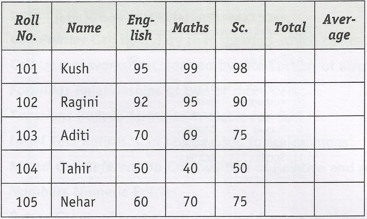
Create the following worksheet in Ooo Calc :
Answer
Below is the created worksheet in Ooo Calc:

From the above created worksheet find out the average marks for the entire class using appropriate formulas.
Answer
The average marks for the entire class is 75.2.

We follow the following steps to find the average marks for the entire class:
Step 1 — Find the total marks for each student.
Select F2 and write the formula =SUM(C2 : E2). This formula will calculate the total marks of a student.
With F2 selected, dragging the cell handle from F3 to F6 will copy the formula to the cell range [F3 : F6].
Step 2 — Find the average marks for each student.
Select G2 and write the formula =AVERAGE(C2 : E2). This formula will calculate the average marks of a student.
With G2 selected, dragging the cell handle from G3 to G6 will copy the formula to the cell range [G3 : G6].
Step 3 — Find the average marks for the entire class.
Select cell G8 and write the formula =AVERAGE(G2 : G6).
Now copy the range consisting of the mentioned entire data (including total, average & class average) to a new location. Find out whether the cell references in formulas change or not.
Answer
When we copy the range consisting of the mentioned entire data to a new location, the cell references in the formulas change according to the position of the cells to which they refer.
Now move the original data range (including total, average and class average) to a new location. Find out whether the cell references in formulas change or not.
Answer
When we move the original data range to a new location, the cell references in the formulas change according to the position of the cells to which they refer.
Now move back the moved data range to the original position and make changes in the marks obtained by students. Notice total, average and class average. What happens ? Why does this happen ? What is this feature called ?
Answer
When we move back the moved data range to the original position and make changes in the marks obtained by students, the Total, Average, and Class Average values will automatically update to reflect the changes. This behavior is known as "relative referencing" i.e., the cell references within the formula are adjusted based on their relative positions when we copy or move the formula to different cells.
When we make changes to the marks obtained by students, the formulas for Total, Average, and Class Average are using relative references to the cells containing the student's marks. As a result, when we move the data range back to the original position, the formulas automatically adjust to reference the correct cells, and the calculations update accordingly.
Write commands for the operations (i) — (ii) based upon the spreadsheet shown below :
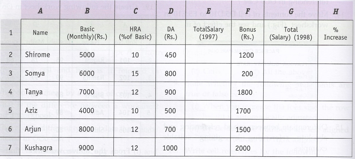
(i) To calculate the total salary as sum of Basic Salary, HRA and DA for each employee for the year 1997.
(ii) To calculate the total salary of each employee for the year 1998 as sum of salary for the year 1997 and bonus. Also calculate the percentage increase in the total salary from 1997 to 1998 for each employee.
Answer
(i) To calculate the total salary as sum of Basic Salary, HRA and DA for each employee for the year 1997, follow the given steps:
Step 1 — Select E2 and write the formula =B2+(C2/100*B2)+D2. This formula will calculate the total salary of Shirome.
Total salary = Basic Pay + HRA + DA
To calculate HRA, we use the formula = C2/100 * B2
Thus, the formula for Total salary =B2+(C2/100*B2)+D2
Step 2 — With E2 selected, dragging the cell handle from E3 to E7 will copy the formula to the cell range [E3 : E7]. The total salary of each employee will be displayed in the respective cell.

(ii) To calculate the total salary of each employee as sum of salary for the year 1997 and bonus, follow the given steps:
Step 1 — Select G2 and write the formula =SUM(E2 : F2). This formula will calculate the total salary (1998) of Shirome.
Step 2 — With G2 selected, dragging the cell handle from G3 to G7 will copy the formula to the cell range [G3 : G7]. The total salary of each employee will be displayed in the respective cell.
To calculate the percentage increase in the total salary from 1997 to 1998 for each employee, follow the given steps:
Step 1 — Select H2 and type the formula =(G2-E2)/E2 * 100.
Step 2 — With H2 selected, dragging the cell handle from H3 to H7 will copy the formula to the cell range [H3 : H7]. The percentage increase in the total salary from 1997 to 1998 for each employee will be displayed in the respective cell.

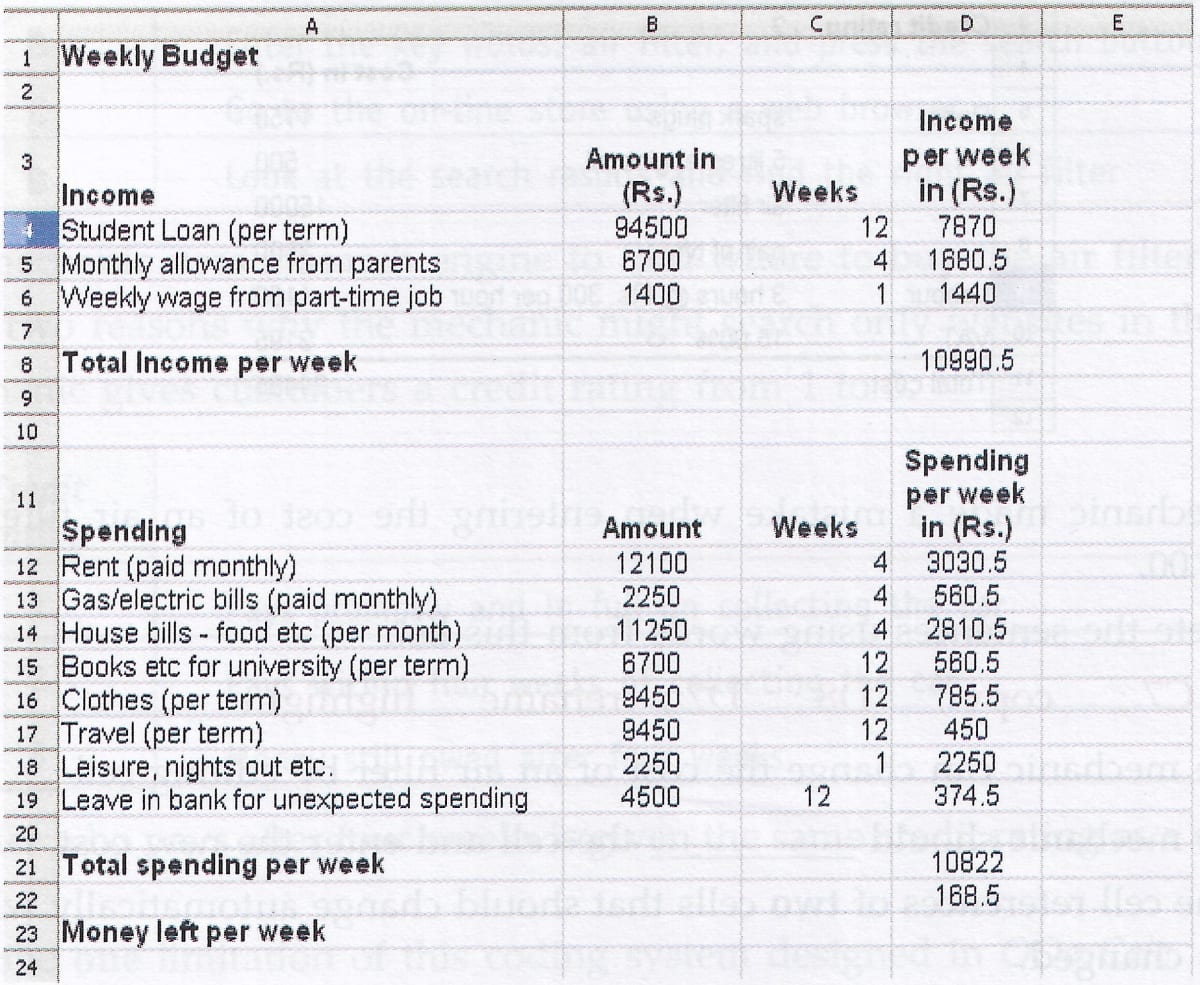
A university student uses a PC to help plan a budget for the first term. Their first attempt is shown below.
(a) Tick one box to show which type of software package has been used.
| Tick one box only | |
|---|---|
| Graphics | |
| Database | |
| Spreadsheet | |
| Multimedia |
(b) Which cell contains the spending on rent per week ?
(c) Which one of the following is the formula used in cell D23 ?
| Tick one box only | |
|---|---|
| = D21 - D8 | |
| = D8 - D21 | |
| = sum(D2 : D12) |
(d) Tick one box to show a disadvantage of using a software package to help work out the budget rather than using a calculator, pen and paper.
| Tick one box only | |
|---|---|
| The formulae could be wrong | |
| The wrong prices could be input | |
| A virus may corrupt the information | |
| Multiple printouts could be produced |
Answer
(a)
| Tick one box only | |
|---|---|
| Graphics | |
| Database | |
| Spreadsheet | ✓ |
| Multimedia |
(b) D12
(c)
| Tick one box only | |
|---|---|
| = D21 - D8 | |
| = D8 - D21 | ✓ |
| = sum(D2 : D12) |
(d)
| Tick one box only | |
|---|---|
| The formulae could be wrong | |
| The wrong prices could be input | |
| A virus may corrupt the information | ✓ |
| Multiple printouts could be produced |
A self-employed car mechanic uses a spreadsheet to calculate bills for customers.
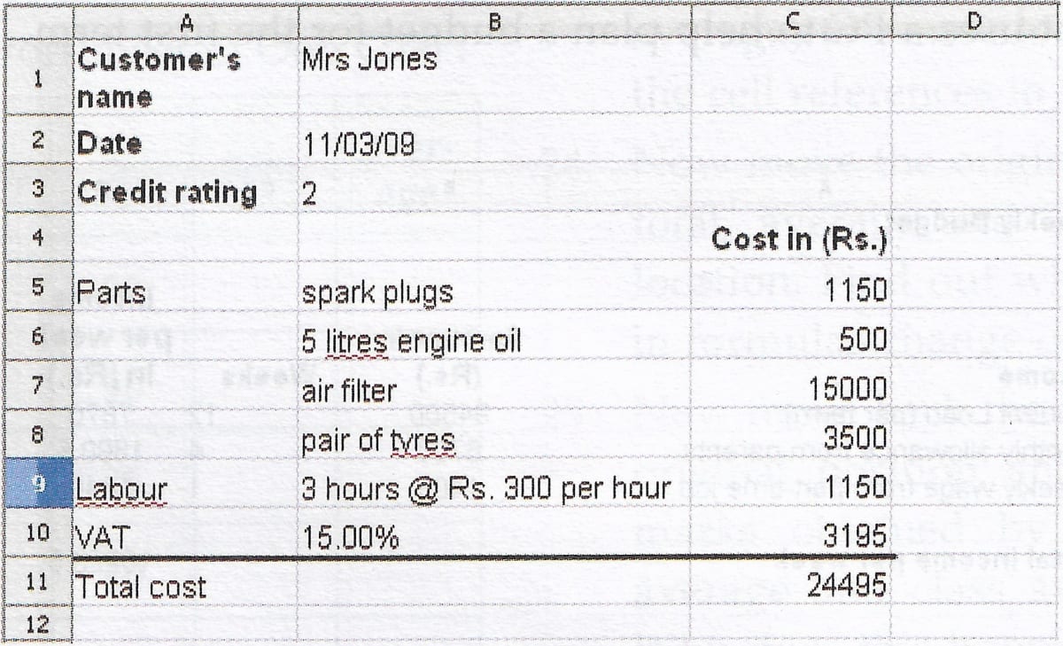
(a) The mechanic made a mistake when entering the cost of an air filter. An air filter costs Rs. 400.00.
Complete the sentences using words from this list.
C7 ; copy ; D8 ; D7 ; rename ; highlight
(i) The mechanic can change the cost of an air filter by editing cell .................. .
(ii) The mechanic should .................. the cell and enter the new cost.
(b) Give the cell references of two cells that should change automatically when the cost of an air filter is changed.
(c) Cells can contain numbers or text.
Tick three boxes to show other types of information a cell can contain.
| Tick three boxes | |
|---|---|
| Printer | |
| Website address | |
| Idea | |
| Formula | |
| Picture | |
| Word processor |
(d) On-line help is available within the spreadsheet.
Tick three boxes to show what should be in the on-line help for the spreadsheet.
| Tick three boxes | |
|---|---|
| A lesson on percentages so the mechanic can calculate VAT | |
| An index to help the mechanic find the information needed | |
| A road map to help the mechanic find the route to the parts warehouse | |
| A tutorial guide to help the mechanic use the spreadsheet | |
| A dictionary that helps the mechanic understand the meaning of words | |
| A search engine to help the mechanic find the information needed |
(e)
(i) The mechanic has to buy the air filter from an on-line store.
Write the labels in order to show how the mechanic can do this.
| Label | |
|---|---|
| A | Pay using a credit card |
| B | Enter the key words: air filter, and press the search button |
| C | Go to the on-line store using a web browser |
| D | Look at the search results and find the right air filter |
(ii) The mechanic uses a search engine to find where to buy the air filter.
State two reasons why the mechanic might search only websites in the India.
(f) The mechanic gives customers a credit rating from 1 to 3.
| Credit Rating | |
|---|---|
| 1 | Pays promptly and in full on collecting the car |
| 2 | Pays within four weeks of collecting the car |
| 3 | Money still owed after four weeks |
A customer who pays after four weeks is given the same credit rating as a customer who does not pay.
(i) Describe one limitation of this coding system designed in OOo Calc.
(ii) Design an improved coding system, if possible.
Answer
(a)
(i) The mechanic can change the cost of an air filter by editing cell C7.
(ii) The mechanic should highlight the cell and enter the new cost.
(b) The two cells that should change automatically when the cost of an air filter is changed are C10 and C11.
(c)
| Tick three boxes | |
|---|---|
| Printer | |
| Website address | ✓ |
| Idea | |
| Formula | ✓ |
| Picture | ✓ |
| Word processor |
(d)
| Tick three boxes | |
|---|---|
| A lesson on percentages so the mechanic can calculate VAT | |
| An index to help the mechanic find the information needed | ✓ |
| A road map to help the mechanic find the route to the parts warehouse | |
| A tutorial guide to help the mechanic use the spreadsheet | ✓ |
| A dictionary that helps the mechanic understand the meaning of words | |
| A search engine to help the mechanic find the information needed | ✓ |
(e)
(i) The mechanic can buy an air filter in the following manner:
C — Go to the on-line store using a web browser
B — Enter the key words: air filter, and press the search button
D — Look at the search results and find the right air filter
A — Pay using a credit card
(ii) Two reasons the mechanic might search only websites in the India are :
- Local Compatibility — Searching for websites within India ensures that the mechanic finds options that are specifically designed to fit vehicles commonly used in the Indian market.
- Get the best price and faster delivery — By focusing on websites within India, the mechanic will avoid import duties so he can get the air filter at the best price. Also shipping time from suppliers within India will be less compared to overseas suppliers.
(f)
(i) One limitation of the coding system described in the scenario is that it lacks differentiation between different levels of late payments. In this system, both a customer who pays after four weeks and a customer who doesn't pay at all are given the same credit rating of 3. It fails to distinguish between a customer who eventually pays but is consistently late and a customer who doesn't pay at all.
(ii) An improved coding system could address this limitation by incorporating more levels of credit ratings to reflect different degrees of payment behavior. Here's a possible improved coding system:
| New Credit Rating | Description |
|---|---|
| 1 | Pays promptly and in full on collecting the car |
| 2 | Pays within two weeks of collecting the car |
| 3 | Pays within four weeks of collecting the car |
| 4 | Pays within six weeks of collecting the car |
| 5 | Pays after six weeks but within two months |
| 6 | Money still owed after two months |
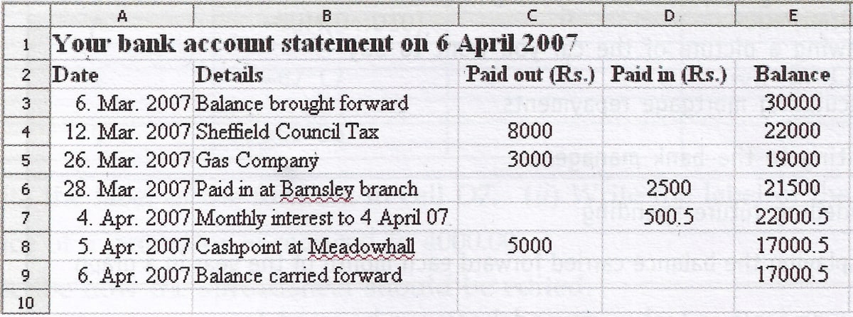
A customer downloads a bank account statement from an online bank.
The statement is downloaded into a spreadsheet.
(a) Tick three boxes to show what can be contained in a cell in a spreadsheet.
| Tick three boxes | |
|---|---|
| A mouse | |
| A date | |
| A number | |
| A website | |
| A picture | |
| A word processor |
(b) The cell reference of the cell which contains 'Balance brought forward' is B3.
- Write down the cell reference of the cell which contains .'Gas Company'.
- Write down the cell reference of the cell which contains .'Paid out'.
(c) Tick one box to show the formula contained in cell E6.
| Tick one box only | |
|---|---|
| =E6 + C6 + D6 | |
| =E5 - C6 + D6 | |
| =D5 + D6 + D7 | |
| =E5 * C6 * D6 | |
| =E5 + C5 + D5 |
(d) Tick one box to show the formula contained in cell E9.
| Tick one box only | |
|---|---|
| =E8 | |
| =E8 - C8 + D8 | |
| =E7 * C8 * D8 | |
| =E8 + D8 | |
| =E8 - C8 |
(e) (i) Tick three boxes to show what a spreadsheet should be used for.
| Tick three boxes | |
|---|---|
| Controlling output from a scanner | |
| Drawing a picture of the car you want to buy | |
| Calculating mortgage repayments | |
| Writing to the bank manager | |
| Modelling future spending | |
| Displaying the balance carried forward each month of the year in a graph |
(ii) State one other task a spreadsheet can be used for.
(f) The customer is using a word processor to fill in a tax return.
The customer needs to copy the monthly interest into the tax return.
Write down the labels in order to show how cell D7 could be copied into the tax return.
| Label | |
|---|---|
| A | Position the cursor in the word processor |
| B | Select copy |
| C | Select paste |
| D | Highlight D7 in the spreadsheet |
(g) The customer saves the statement on a flash memory stick. Give one reason why this may not be secure and suggest a way to make the statement more secure.
(h) Tick one box to show how much space the spreadsheet file (.ods) is likely to use on backing storage.
| Tick one box only | |
|---|---|
| 150 Megabytes | |
| 80 Gigabytes | |
| 15 Kilobytes | |
| 10 bytes | |
| 0 bytes |
Answer
(a)
| Tick three boxes | |
|---|---|
| A mouse | |
| A date | ✓ |
| A number | ✓ |
| A website | |
| A picture | ✓ |
| A word processor |
(b)
- The cell which contains 'Gas Company' is B5.
- The cell which contains 'Paid out' is C2.
(c) Formula contained in cell E6:
| Tick one box only | |
|---|---|
| =E6 + C6 + D6 | |
| =E5 - C6 + D6 | ✓ |
| =D5 + D6 + D7 | |
| =E5 * C6 * D6 | |
| =E5 + C5 + D5 |
(d) Formula contained in cell E9:
| Tick one box only | |
|---|---|
| =E8 | ✓ |
| =E8 - C8 + D8 | |
| =E7 * C8 * D8 | |
| =E8 + D8 | |
| =E8 - C8 |
(e)
(i) A spreadsheet should be used for:
| Tick three boxes | |
|---|---|
| Controlling output from a scanner | |
| Drawing a picture of the car you want to buy | |
| Calculating mortgage repayments | ✓ |
| Writing to the bank manager | |
| Modelling future spending | ✓ |
| Displaying the balance carried forward each month of the year in a graph | ✓ |
(ii) Spreadsheet can also be used to compute and manage student grades for academic purposes.
(f) To copy the monthly interest from cell D7 into the tax return, follow the given steps:
D — Highlight D7 in the spreadsheet
B — Select copy
A — Position the cursor in the word processor
C — Select paste
(g) Storing a bank statement on a flash memory stick may not be secure due to the risk of physical loss or theft. If the memory stick is misplaced or stolen, unauthorized individuals could gain access to sensitive financial information.
To make the statement more secure, use password protection. To set a password for an OOo Calc document, follow the given steps:
Step 1 — Open the statement in OOo Calc.
Step 2 — Go to "File" > "Save As."
Step 3 — In the "Save As" dialog box, check the "Save with password" option.
Step 4 — Enter and confirm your desired password.
Step 5 — Save the document.
(h) Space used by spreadsheet file (.ods) on backing storage:
| Tick one box only | |
|---|---|
| 150 Megabytes | |
| 80 Gigabytes | |
| 15 Kilobytes | ✓ |
| 10 bytes | |
| 0 bytes |
A finance officer uses a spreadsheet to record sales from an equipment shop. This is part of the spreadsheet.
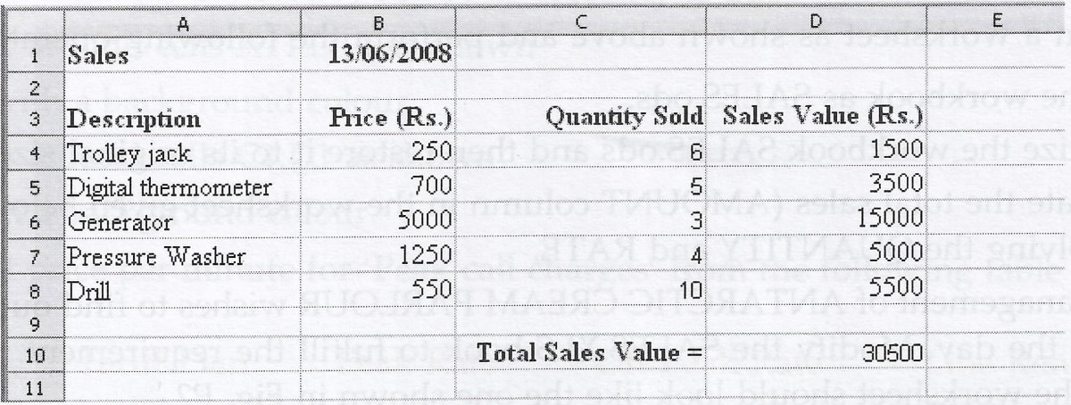
(a)
| Label | Formula | Label | Formula |
|---|---|---|---|
| A | =SUM(D4 : D10) | D | =SUM(D4 : D8) |
| B | =B7 * C7 | E | =A7 * B7 * C7 |
| C | =C6 * D6 |
- Write the label of the formula in cell D7.
- Write the label of the formula in cell D10.
(b) The price of a generator is reduced to 4000.00.
- Describe how the spreadsheet should be edited.
- When the spreadsheet was edited, the values displayed in some cells changed automatically. Write in the box the cell reference of two cell that changed automatically.
- Tick one box to show why a cell would change automatically when another cell is edited.
| Tick one box only | |
|---|---|
| Spreadsheet cells are all linked | |
| The cell contains a formula that refers to the other cell | |
| All the cells know what is happening in other cells | |
| The cell contains a description that refers to the other cell | |
| The spreadsheet contains a graph |
Answer
(a)
- The label of the formula in cell D7 is B.
- The label of the formula in cell D10 is D.
(b)
To edit the price of the generator, follow the given steps:
Step 1 — Select cell B6.
Step 2 — Type '4000' in the cell. The previous value (5000) will be overwritten.
The formula of cell D6 (= B6 * C6) will automatically update the sales value in the spreadsheet.D6 and D10.
Reason for cell updating automatically:
| Tick one box only | |
|---|---|
| Spreadsheet cells are all linked | |
| The cell contains a formula that refers to the other cell | ✓ |
| All the cells know what is happening in other cells | |
| The cell contains a description that refers to the other cell | |
| The spreadsheet contains a graph |