What is the default format for expressing numbers in Excel?
- General
- Percent
- -1234
- User-defined
Answer
General
Reason — General is the default format for expressing numbers in Excel.
Which tab is used to set the horizontal and vertical alignment for data in cells?
- Number
- Font
- Alignment
- Background
Answer
Alignment
Reason — Alignment tab is used to set the horizontal and vertical alignment for data in cells.
Which feature in Excel is used to rotate text through a specified angle?
- Text Orientation
- Text Alignment
- Text Indent
- Text Formatting
Answer
Text Orientation
Reason — Text Orientation feature in Excel is used to rotate text through a specified angle.
Which term is used to define a graphical representation of data in a worksheet?
- Text
- Table
- Cells
- Chart
Answer
Chart
Reason — Chart is used to define a graphical representation of data in a worksheet.
What type of chart is used to emphasize the magnitude of change over time?
- Pie
- Area
- Bar
- Scatter
Answer
Area
Reason — Area chart is used to emphasize the magnitude of change over time.
............... chart is designed specifically for plotting data values related to stocks and shares.
- Pie
- Area
- Bar
- Stock
Answer
Stock
Reason — Stock chart is designed specifically for plotting data values related to stocks and shares.
In which group of the Home tab is the Format option available?
- Clipboard
- Cells
- Font
- Number
Answer
Cells
Reason — The Format option is available in the Cells group of the Home tab.
Name the type of chart which displays data in the form of a circle.
- Pie
- Area
- Bar
- Scatter
Answer
Pie
Reason — Pie chart displays data in the form of a circle.
What is the name for the horizontal axis of a chart?
- Y-axis
- Legend
- Value axis
- Category axis
Answer
Category axis
Reason — The horizontal axis of a chart is called Category axis.
Which component in Excel helps in depicting colors, patterns or symbols assigned to data series?
- Font
- Legend
- Data Range
- Chart Area
Answer
Legend
Reason — Legend component helps in depicting colors, patterns or symbols assigned to data series.
Which type of chart is used for representing huge amount of data?
- Pie
- Line
- Bar
- Scatter
Answer
Line
Reason — Line chart is used for representing huge amount of data.
What is the other name for XY chart?
- Pie
- Area
- Bar
- Scatter
Answer
Scatter
Reason — Scatter is the other name for XY chart.
When a chart is placed inside a worksheet along with its source data, it is called ................ .
- Chart Wall
- Embedded Chart
- Chart Sheet
- Chart Area
Answer
Embedded Chart
Reason — When a chart is placed inside a worksheet along with its source data, it is called Embedded Chart.
Name the item that forms the heading of a chart.
- Legend
- Subtitle
- Value axis
- Chart Title
Answer
Chart Title
Reason — Chart Title forms the heading of a chart.
The first Pie chart was seen in William Playfair's book of 'Statistical Breviary' in ............... .
- 1908
- 1802
- 1805
- 1801
Answer
1801
Reason — The first Pie chart was seen in William Playfair's book of 'Statistical Breviary' in 1801.
Name the type of chart which does not have grid lines.
- Line
- Bar
- Pie
- Column
Answer
Pie
Reason — Pie chart does not have grid lines.
............... is called the total area of the chart.
- Data Area
- Plot Area
- Chart Area
- None of these
Answer
Chart Area
Reason — Chart Area is the total area of the chart.
In MS Excel, Charts group is available on the ............... tab.
- Home
- Data
- Insert
- Formulas
Answer
Insert
Reason — In MS Excel, Charts group is available on the Insert tab.
The axis that represents the values or units of the source data is called ............... .
- Category Axis
- Axis
- Value Axis
- None of these
Answer
Value Axis
Reason — The axis that represents the values or units of the source data is called Value Axis.
Which type of chart looks similar to a spider net?
- Pie
- Bar
- Column
- Radar
Answer
Radar
Reason — Radar chart looks similar to a spider net.
You can change the font size of text within a cell.
Answer
True
Reason — We can change the font size of text within a cell.
Text cannot be aligned within a cell.
Answer
False
Reason — Text can be aligned within a cell both horizontally and vertically.
The default format for expressing numbers in Excel is general.
Answer
True
Reason — The default format for expressing numbers in Excel is general.
The number of decimal places to be displayed can be increased or decreased in Excel.
Answer
True
Reason — The number of decimal places to be displayed can be increased or decreased from the Number Format box in the Number group on the Home tab.
The Alignment tab is used to set only the horizontal alignment for data in cells.
Answer
False
Reason — The Alignment tab is used to set both the horizontal alignment as well as vertical alignment of data in cells.
Justified option aligns data in cell to the left and to the right borders.
Answer
True
Reason — Justified option aligns data in cell to the left and to the right borders.
Text Orientation is used to rotate text through a specified angle.
Answer
True
Reason — Text Orientation is used to rotate text through a specified angle.
We cannot change the font color of data within the cells.
Answer
False
Reason — We can change the font color of data within the cells from the Font Color option present in the Font group of Home tab.
A chart is a textual representation of data in a worksheet.
Answer
False
Reason — A chart is a graphical representation of data in a worksheet.
Area chart displays data in the form of long rectangular rods also called bars.
Answer
False
Reason — Area chart emphasizes the magnitude of change over time. By showing the sum of the plotted values, an Area chart displays the relationship of parts to the whole.
Line chart is in the form of lines and is used to illustrate trends in data at equal intervals.
Answer
True
Reason — Line chart is in the form of lines and is used to illustrate trends in data at equal intervals.
Scatter chart is the default chart type in Excel.
Answer
False
Reason — Column chart is the default chart type in Excel.
Stock chart has been designed specifically for plotting data related to stocks and shares.
Answer
True
Reason — Stock chart has been designed specifically for plotting data related to stocks and shares.
Page Preview is used to check the overall content and formatting of a worksheet.
Answer
True
Reason — Page Preview is used to check the overall content and formatting of a worksheet.
The shortcut key to preview the worksheet is Ctrl + F2.
Answer
True
Reason — The shortcut key to preview the worksheet is Ctrl + F2.
There are only two types of charts in Excel.
Answer
False
Reason — There are eleven types of charts commonly used in Excel.
MS Excel does not have option to preview the worksheet before sending it to print.
Answer
False
Reason — Ctrl + F2 key combination can be used to show the print preview of the worksheet.
A Pie chart compares pieces of data using horizontal stacks.
Answer
False
Reason — A pie chart displays data in the form of a circle that is divided into a series of segments. It shows the proportional size of individual items that makes up a data series to the sum of items.
Chart represents only pictorial information.
Answer
False
Reason — A chart is a graphical representation of data in a worksheet. It helps to provide a better understanding of large quantities of data. Charts make it easier to draw comparison and see growth, relationship among the values and trends in data.
The Doughnut chart displays data in the form of bars.
Answer
False
Reason — The Doughnut chart displays data as sections of a circle. It can have more than one data series, which attempts to add another dimension to the Pie chart.
What do you understand by text orientation?
Answer
Text Orientation is used to rotate text through a specified angle. Text can be oriented in both up and down directions by specifying the angle in degrees.
Which formatting effects can you apply using the Home tab? Explain a few.
Answer
Home tab provides us access to many groups which can be used to apply various formatting effects. Some of the formatting effects are as follows:
- Formatting Numbers — Numbers in Excel can be presented in different formats. By default, numbers are expressed in General format. The other formats for numbers are number, currency, accounting, date, time, percentage, fraction etc.
- Change Font — MS Excel offers Font option in the Font group to change the font of text.
- Change Font Size — MS Excel offers Size option in the Font group to change the font size of text.
- Font Style — MS Excel offers three font styles — Bold, Italics and Underline to emphasize the text.
- Cell Alignment — We can change the cell alignment in both ways i.e horizontally as well as vertically from the Alignment group of the Home tab.
- Text Alignment — It is used to align the text vertically and horizontally. Vertical alignment has the options — top, middle and bottom. Horizontal alignment has the options — left, center and right.
Define the term chart. Name any two types of charts.
Answer
A chart is a graphical representation of data in a worksheet. It helps to provide a better understanding of large quantities of data.
Two types of charts are:
- Bar chart
- Pie chart
Differentiate between Category Axis and Value Axis.
Answer
| Category Axis | Value Axis |
|---|---|
| Category axis or X-axis is the horizontal axis of a chart. | Value axis or Y-axis is the vertical axis used to plot the values. |
| It is located at the bottom of the chart. | It is located at the left side of the chart. |
Name the option which is used to see the output before printing. How is it used in Excel?
Answer
Print Preview option is used to see the output before printing.
To view the print preview of the spreadsheet, we follow the steps given below:
Step 1 — Click on the File tab and select the Print option.
Step 2 — A preview of worksheet automatically appears on the right side of the 'Print' pane.
Step 3 — If the worksheet contains more than one page, then click on the Next Page or Previous Page arrow buttons present at the bottom of the Preview window.
Step 4 — To exit Print Preview, simply press the Esc key
What is a Scatter chart?
Answer
Scatter chart either shows the relationships in several data series or plots two groups of numbers as one series of XY co-ordinates. This chart shows uneven intervals or cluster of data and is commonly used for displaying scientific data.
X axis is usually assigned to an independent variable, the variable whose value is controlled or set by the experimenter. The Y variable then becomes the dependant variable. Its each value depends upon the corresponding value of variable X.
Define Embedded Chart.
Answer
Excel offers the features to create an Embedded chart in a worksheet. It is displayed along with source data and other information present in a worksheet. An embedded chart is saved with the corresponding worksheet when a workbook is saved.
What is the difference between Radar chart and Stock chart?
Answer
| Radar chart | Stock chart |
|---|---|
| Radar chart looks similar to a spider net. It displays data values plotted as points which are connected by lines to form a grid. | Stock chart is a type of column graph, which has been designed specifically for plotting data values related to stocks and shares or fluctuation of daily or annual temperature. |
| It is useful for comparing data that is not time dependent, but shows different circumstances such as variables in a scientific experiment or direction. | The data required for these charts consists of specific data series like opening price, closing price, and high and low prices. |
| The poles of the Radar chart are equivalent to the Y-axis of other charts. | In this type of chart, the X-axis represents a time series. |
Explain the different components of a chart.
Answer
The different components of a chart are as follows:
- Chart Area — Chart area includes all the area and objects in the chart.
- Category Axis — Category axis or X-axis is the horizontal axis of a chart.
- Value Axis — Value axis or Y-axis is the vertical axis used to plot the values. It is located at the left side.
- Data Series — Data series are the bars, slices or other elements that show the data values. If there are multiple data series in the chart, each will have a different colour or style.
- Category Name — Category names are the labels, which are displayed on the X and Y axis.
- Plot Area — Plot area is a window within the Chart area. It contains the actual chart itself and includes plotted data, data series, category, and value axis.
- Legend — It depicts the colours, patterns, or symbols assigned to the data series. It helps to differentiate the data.
- Chart Title — It describes the aim and contents of the chart.
- Gridlines — These can either be horizontal or vertical lines depending on the selected chart type. They extend across the plot area of the chart. Gridlines make it easier to read and understand the values.
What is Pie chart? Describe its features.
Answer
Pie chart displays data in the form of a circle that is divided into a series of segments.
The features of a Pie chart are as follows:
- It shows the proportional size of individual items that makes up a data series to the sum of items.
- It always shows only one data series and is useful when we want to emphasize on a significant element.
- This chart works best with smaller number of values.
Explain the process of printing a complete workbook.
Answer
We follow the given steps to print a complete workbook:
Step 1 — Click the File tab and select Print to access the Print pane.
Step 2 — Select the option Print Entire Workbook from the print range drop-down menu in the Settings section.
Step 3 — Change the page orientation either Portrait or Landscape from the Orientation drop-down list.
Step 4 — Choose the printer from the Printer drop-down list.
Step 5 — Enter the number of copies in the Copies spin box.
Step 6 — After selecting all the required options, click on the Print button.
The entire workbook will be printed.
Describe the text formatting features of MS Excel and how are these useful.
Answer
MS Excel offers various formatting features to improve the appearance of text. You can change the text alignment, font, color, size, style, etc. through the formatting effects available in MS Excel. The text formatting features are as follows:
- Font Styles and Sizes — Excel allows users to customize text with various font styles and sizes, facilitating emphasis on specific information.
- Bold, Italics, and Underline — Users can apply these formatting options to highlight or differentiate data, making it visually appealing and easier to read.
- Text Alignment — Excel provides options for aligning text within cells, such as left, right, center, or justified, improving the overall presentation of data.
- Cell Merging and Wrapping — Merging cells creates custom layouts, while text wrapping ensures that lengthy text fits within a cell, preventing overflow and maintaining a tidy appearance.
- Text Orientation — This feature is used to rotate the text through a specified angle. Tilting text at an angle can enhance the visibility of data labels and can contribute to the overall aesthetics of the spreadsheet.
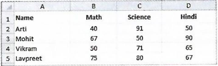
A chart displaying the subject wise attendance of four students and its source data have been given to you. Answer the following questions based on them:
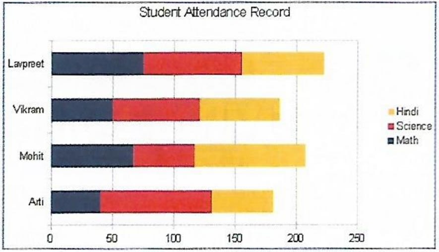
(i) Identify the Type of chart.
(ii) What is the title of the chart?
(iii) List the cell references of the three cell ranges used to produce this chart.
(iv) Suggest a suitable label for both category axis and value axis.
Answer
(i) The given chart is a type of stacked bar chart.
(ii) The title of the chart is 'Student Attendance Record'.
(iii) The cell references of the three cell ranges used to produce this chart are:
- B2 : B5
- C2 : C5
- D2 : D5
(iv) A suitable label for Category Axis can be 'Student Name'.
A suitable label for Value Axis can be 'Number of Days'.
A table containing descriptions of different types of charts is given below. Names of some charts are given below within the bracket. Fill them in front of their respective descriptions and complete the assignment.
[Stock, Area, Bar, Pie, Line, and Radar]
| Name | Description |
|---|---|
| It displays data in the form of long rectangular rods also called bars. | |
| This chart displays data in the form of a circle. | |
| It emphasizes the magnitude i.e., the volume of change over time. | |
| It is designed specifically for plotting data values related to stocks and shares. | |
| It is in the form of lines and is used to illustrate trends in data at equal intervals. | |
| It is a type of chart that resembles a spider net. |
Answer
| Name | Description |
|---|---|
| Bar | It displays data in the form of long rectangular rods also called bars. |
| Pie | This chart displays data in the form of a circle. |
| Area | It emphasizes the magnitude i.e., the volume of change over time. |
| Stock | It is designed specifically for plotting data values related-to stocks and shares. |
| Line | It is in the form of lines and is used to illustrate trends in data at equal intervals. |
| Radar | It is a type of chart that resembles a spider net. |
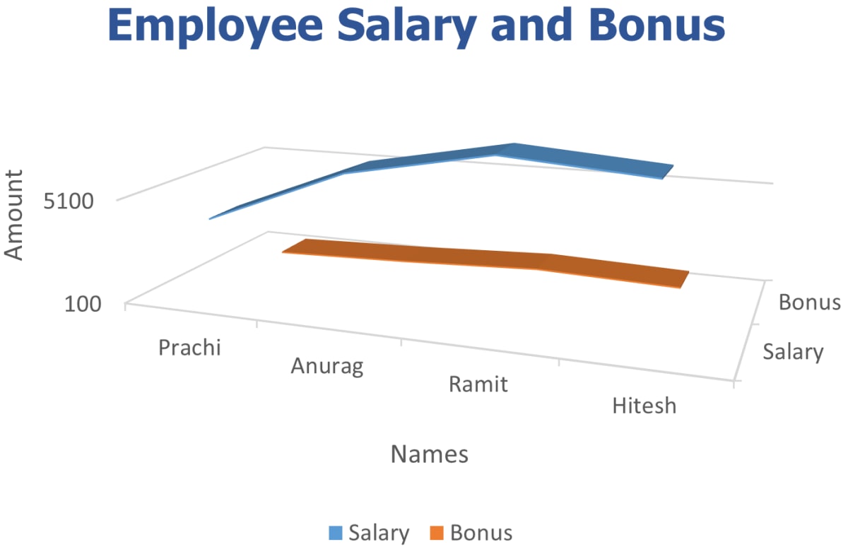
A 3D line chart on Employee Payroll System is given below. Apply the following formatting effects to the chart:
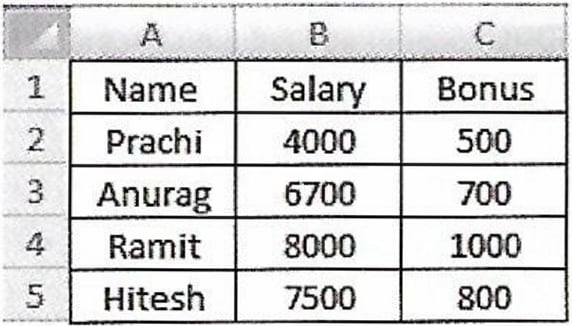
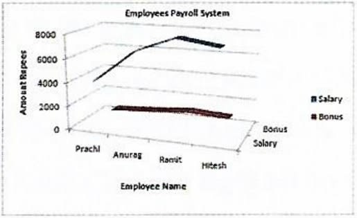
(i) Change the Chart Title to 'Employee Salary and Bonus'.
(ii) Change the title of X axis to 'Names' and Y axis to 'Amount'.
(iii) Change the Font of Chart Title to 'Tahoma', Font size as 16, Font style as Bold and Font color as blue.
(iv) Change the scale for Y axis and display the values between 100 to 8500.
Answer
(i) We can follow the given steps to change the chart title:
Step 1 — Double-click on the chart title.
Step 2 — A textbox appears around the title.
Step 3 — Delete the previous title and type 'Employee Salary and Bonus' in the text box.
Step 4 — Click outside the chart area and the Chart Title will be changed.
(ii) We can follow the given steps to change the title of X axis:
Step 1 — Double-click on the title of X axis.
Step 2 — A textbox appears around the title.
Step 3 — Delete the previous title and type 'Names' in the text box.
Step 4 — Click outside the chart area and the title of X axis will be changed.
Similarly, the title of Y-axis can be changed by clicking on the title of Y axis and replacing the previous title with 'Amount' in the text box.
(iii) We can follow the given steps to format the Chart Title:
Step 1 — Click on the chart title and select it.
Step 2 — Go to the 'Home' tab on the Excel ribbon.
Step 3 — Use the Font options to change the font to 'Tahoma', size to 16, style to Bold, and color to blue.
(iv) We can follow the given steps to change the scale for Y axis and display the values between 100 to 8500:
Step 1 — Click on the chart to select it.
Step 2 — Point the mouse at Y-axis. Right-click on it and select the Format Axis option from the Shortcut menu.
Step 3 — The Format Axis dialog box will open. The Axis Options tab is selected by default. Click on the Fixed radio button for Minimum field and enter 100 in the text box.
Step 4 — Similarly, enter 8500 in the text box of the Maximum field. Click on Close button. The scale on the chart changes accordingly.
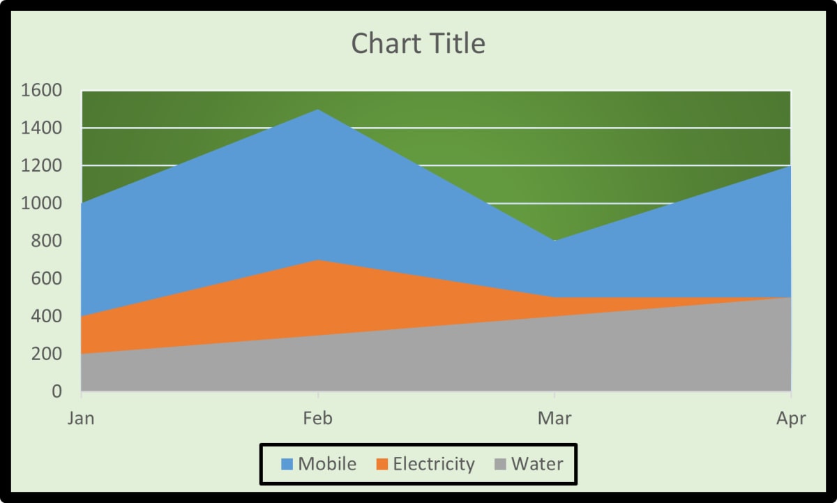
An Area chart depicting the trends in Bills over different months is shown along with its source data. Apply the formatting effects given below to the Area chart then print this chart along with the worksheet data.
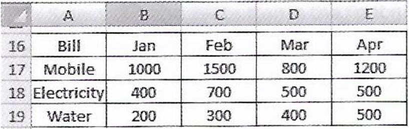
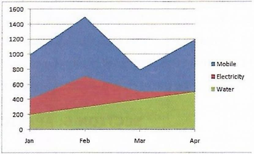
(i) Apply a border to the Chart area and also apply a background color of your choice.
(ii) Using the Gradient Fill option, set the background for the Plot area as 'Moss'.
(iii) Apply a border to the Legend and position it at the bottom of the chart.
Answer
(i) We can follow the given steps to apply a border to the chart area:
Step 1 — Right-click on the Plot area and select the Format Plot Area option. The Format Plot Area dialog box appears.
Step 2 — Select 'Border Styles', 'Border Color', 'Shadow', etc.
Step 3 — By default, the Fill tab is selected. Select the Solid fill option in the right pane.
Step 4 — Click on the Color button and select the desired colour from the drop down menu.
Step 5 — Click on Close button.
We can follow the given steps to apply a background color of our choice:
Step 1 — Click on the chart to select it.
Step 2 — Right-click and choose "Format Chart Area."
Step 3 — In the Format Chart Area pane, choose 'Fill & Line.'
Step 4 — Click on 'Fill' and choose the background color.
(ii) We can follow the given steps to set the background for the Plot area as 'Moss':
Step 1 — Click on the plot area of the chart.
Step 2 — Right-click and choose "Format Plot Area."
Step 3 — In the Format Plot Area pane, go to the Fill options.
Step 4 — Choose 'Gradient Fill' and set the gradient colors, selecting 'Moss' as one of the colors.
(iii) We can follow the given steps to apply a border to the Legend and position it at the bottom of the chart:
Step 1 — Click on the legend to select it.
Step 2 — Right-click and choose "Format Legend."
Step 3 — In the Format Legend pane, go to the Border Color option and choose a border color. Adjust the Border Styles and Weight as needed.
Step 4 — To position the legend at the bottom, right-click and choose 'Legend Options'.
Step 5 — Click on Bottom in the Position option.