Microsoft Excel 2010 - I

Multiple Choice Questions

Question 1

Which software lets you perform calculations and manipulate the numeric data?

1. MS Excel
2. MS Word
3. MS PowerPoint
4. All of these

Answer

MS Excel

Reason — MS Excel lets us perform calculations and manipulate the numeric data.

Question 2

Name the element which is identified by a unique row number and column number.

1. Cell
2. Column
3. Row
4. None of these

Answer

Cell

Reason — Cell is the element which is identified by a unique row number and column number.

Question 3

What do we call a group of contiguous cells which form the shape of a rectangle?

1. Cell
2. Spreadsheet
3. Range
4. SheetTab

Answer

Range

Reason — Range is a group of contiguous cells which form the shape of a rectangle.

Question 4

Which symbol separates the address of the starting cell address from the ending cell address in a range?

1. Semicolon
2. Colon
3. Full Stop
4. None of these

Answer

Colon

Reason — Colon symbol separates the address of the starting cell address from the ending cell address in a range.

Question 5

Which of the following component lies at the top of the document window in MS Excel?

1. Task Bar
2. Status Bar
3. Formula Bar
4. Title Bar

Answer

Title Bar

Reason — Title Bar lies at the top of the document window in MS Excel.

Question 6

What name do we give to the current cell which has a cell boundary around it?

1. Passive Cell
2. Active Cell
3. Current Cell
4. New Cell

Answer

Active Cell

Reason — Active Cell is the current cell which has a cell boundary around it.

Question 7

Which is the last valid column header in MS Excel?

1. XFD
2. AJ
3. AZ
4. AJM

Answer

XFD

Reason — XFD is the last valid column header in MS Excel.

Question 8

What is the default name of a workbook in MS Excel?

1. Book1
2. Sheet1
3. Untitled1
4. All of these

Answer

Book1

Reason — The default name of a workbook in MS Excel is Book1.

Question 9

Which shortcut key combination is used to save a workbook in MS Excel?

1. Ctrl + X
2. Ctrl + Z
3. Ctrl + C
4. Ctrl + S

Answer

Ctrl + S

Reason — Ctrl + S key combination is used to save a workbook in MS Excel.

Question 10

Which pair of brackets are used to denote a negative value in MS Excel?

1. Parenthesis
2. Curly Brackets
3. Square Brackets
4. All of these

Answer

Parenthesis

Reason — A pair of parenthesis are used to denote a negative values in MS Excel.

Question 11

What is the default alignment for numbers in MS Excel?

1. Left
2. Right
3. Center
4. None of these

Answer

Right

Reason — The default alignment for numbers in MS Excel is right.

Question 12

Name the expression which includes numbers, cell addresses, operators, and parenthesis.

1. Symbol
2. Equation
3. Formula
4. None of these

Answer

Formula

Reason — Formula is the expression which includes numbers, cell addresses, operators, and parenthesis.

Question 13

Which symbol marks the beginning of a formula?

1. Equal (=)
2. Plus (+)
3. Asterik (*)
4. Division (/)

Answer

Equal (=)

Reason — The symbol Equal (=) marks the beginning of a formula.

Question 14

Which data entry is neither a number nor a formula?

1. Date
2. Character
3. Text
4. None of these

Answer

Text

Reason — Text is neither a number nor a formula.

Question 15

By default, how many worksheets does an excel workbook display?

1. 1
2. 2
3. 3
4. 4

Answer

3

Reason — An excel workbook displays 3 worksheets.

Question 16

What separates time elements in Excel?

1. Colons
2. Hyphen
3. Slash
4. Equal to

Answer

Colons

Reason — Colons separate time elements in Excel.

State True or False

Question 1

If we type the apostrophe symbol before a number, Excel assumes it as a text entry.

Answer

True

Reason — If we type the apostrophe symbol before a number, Excel assumes it as a text entry.

Question 2

The date entries in Excel are separated by the colon symbol.

Answer

False

Reason — In Excel, the colon symbol (:) is used to create a range of cells. Date entries in Excel are typically recognized using date formats, such as "mm/dd/yyyy" or "dd-mm-yyyy".

Question 3

The F3 function key is used to edit the contents of the active cell.

Answer

False

Reason — The F2 function key is used to edit the contents of the active cell. Pressing F2 key places the cursor at the end of the cell contents.

Question 4

The Clear All option clears all the contents from the selected range of cell.

Answer

True

Reason — The Clear All option clears all the contents from the selected range of cell.

Question 5

The shortcut key combination to cut a specific range of cells is Ctrl + X.

Answer

True

Reason — The shortcut key combination to cut a specific range of cells is Ctrl + X.

Question 6

The name given to a range of cells is added in the drop-down list of the Name Box.

Answer

True

Reason — The name given to a range of cells is added in the drop-down list of the Name Box.

Question 7

The small black square present in the lower right corner of the active cell is called the Cell Handle.

Answer

True

Reason — The small black square present in the lower right corner of the active cell is called the Cell Handle.

Question 8

The Insert dialog box has four different options to choose from.

Answer

True

Reason — The Insert dialog box has four options to choose from which are as follows:

1. Shift cells right
2. Shift cells down
3. Entire row
4. Entire column

Question 9

The number of blank cells inserted in a worksheet will be same as the number of cells selected initially.

Answer

True

Reason — The number of blank cells inserted in a worksheet will be same as the number of cells selected initially.

Question 10

An expression which includes cell addresses, numbers, operators, and parenthesis is called a Chemical Equation.

Answer

False

Reason — An expression which includes cell addresses, numbers, operators, and parenthesis is called a Formula.

Question 11

Formulas always begin with the '=' symbol followed by cell references and operators.

Answer

True

Reason — Formulas always begin with the '=' symbol followed by cell references and operators.

Question 12

We use the Compound Formulas when we need more than one operator.

Answer

True

Reason — We use the Compound Formulas when we need more than one operator.

Question 13

The other name of cell reference in MS Excel is cell address.

Answer

True

Reason — The other name of cell reference in MS Excel is cell address.

Question 14

Alphanumeric data cannot be entered in a worksheet.

Answer

False

Reason — Numeric, alphanumeric, non-numeric, or formula can be entered in an Excel worksheet. Alphanumeric data refers to text data.

Theory Questions

Question 1

What are functions? Explain the different parts of functions.

Answer

Functions are pre-designed formulas to perform simple and complex calculations.

Functions are made up of two parts:

1. Arguments — Arguments are input values to functions. Arguments can be numbers, text, logical values like True or False, range of cell reference, or formulas that are enclosed within parenthesis.
2. Structure — The Structure of a function defines its basic skeleton, which forms the base of writing general syntax of functions. The structure begins with the equal sign(=), function name and then followed by the list of arguments separated by a comma within the parenthesis.

The syntax of writing a function is as follows:

= FUNCTION NAME (argument1, argument2, argument3... )

Question 2

Can we find the average of more than one range of cells? If yes, what will be the structure of such a function?

Answer

Yes, we can find the average of more than one range of cells by using the AVERAGE function.

The structure of the AVERAGE function used is as follows:

= AVERAGE (Range1 , Range2, ...)

For example, to find out the average of range B2 : D2 and B3 : D3, we will write the formula as follows:

= AVERAGE (B2 : D2 , B3 : D3)

Question 3

What is the significance of COUNT() function? What type of data entries does the COUNT() function recognize?

Answer

The COUNT() function counts the number of numeric entries, formula, and date entries in a given range of cells. It is particularly useful for quickly determining the count of numerical entries in a dataset.

The COUNT() function is significant for statistical analysis and data validation. It helps us understand the size of a dataset, especially when dealing with numerical values.

The COUNT() function recognizes and counts cells that contain numerical values, including integers, decimals, and dates that Excel recognizes as numerical values. It excludes non-numeric entries such as text, errors, and blank cells.

Question 4

Which logical values are recognized by most of the functions? What are the corresponding numeric values of those logical values?

Answer

In Excel, logical values are represented by the TRUE and FALSE values. These logical values are widely recognized by most functions for conditional testing and logical operations. The corresponding numeric values are:

TRUE — corresponds to the numeric value 1.

FALSE — corresponds to the numeric value 0.

When we use TRUE or FALSE in a numeric context, Excel automatically treats them as 1 and 0, respectively.

Question 5

Suggest the Excel functions which can be used for the following:

(a) To calculate the average marks obtained by a student in SA1 assuming that his/her marks of individual subjects are given.

(b) To find the highest marks of Hindi in your class, if marks of all students are given.

(c) To calculate the quarterly sales of a sales executive, if the sales data of all months are given.

(d) To find out the minimum quoted tender rates submitted by various companies to the Govt. of India.

Answer

(a) = AVERAGE ()

(b) = MAX ()

(c) = SUM ()

(d) = MIN ()

Application Based Questions

Question 1

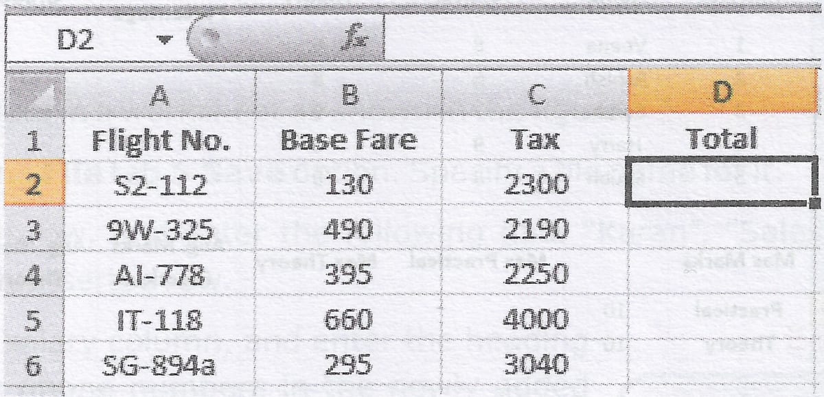
An assignment was given to Sanjiv and Vibha by their teacher. They were shown the screen shot given below and were asked to answer the following questions:

(i) What happens when the formula = B2 + C2 is entered in D2?

(ii) What happens when the formula of D2 is copied over to D6?

(iii) What will happen if we modify the formula in the cell D6 to = $\text{\textdollar B}6 + \text{\textdollar C}6$?

(iv) What happens when we copy the formula of D6 to D3?

(v) If we delete the value of C3, what will be the new value of D3?

Answer

(i) D2 will display the sum of the values in cells B2 and C2.

D2 = B2 + C2
D2 = 130 + 2300
D2 = 2430

(ii) When the formula in D2 is copied over to D6, the relative references in the formula (B2 and C2) will adjust based on the relative position. So, the formula will be modified as = B6 + C6. Thus, D6 will display the sum of the values in cells B6 and C6.

D6 = B6 + C6
D6 = 295 + 3040
D6 = 3335

(iii) The dollar signs $(\text{\textdollar})$ indicate absolute references, meaning that the column (B and C) will remain fixed when the formula is copied or filled to other cells horizontally. The row (6) will still adjust based on the relative position.

(iv) When the formula in D6 is copied to D3, The absolute references (B and C) will remain fixed and only row (6) will adjust according to the relative position.

Thus, the formula in D3 will be $=\text{\textdollar B}3 + \text{\textdollar C}3$, reflecting the change in the row number while keeping the column references fixed.

D3 = $\text{\textdollar B}3 + \text{\textdollar C}3$
D3 = 490 + 2190
D3 = 2680

(v) If the value of C3 is deleted, the new value of D3 will be the sum of the remaining values in B3 and C3 (now treated as 0).

D3 = $\text{\textdollar B}3 + \text{\textdollar C}3$
D3 = 490 + 0
D3 = 490

Question 2

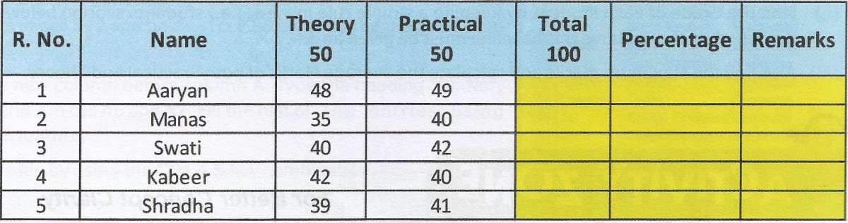
Mayur could not complete the assignment given by his teacher which is shown below. Help him to fill the blank cells marked with yellow colour.

Answer

Mayur can use formulas to calculate the values of the blank cells. Let us assume that "R. No." has the cell reference A1 and write the formulas accordingly.

1. To calculate Total, he can write the formula = C2 + D2 in cell E2. This formula will calculate the sum of cells C2 and D2 in cell E2. The formula can be copied in range E3 : E6 to fill the Total column.

2. To calculate Percentage, he can write the formula = (E2 / 100) * 100 in cell F2. This formula will calculate the percentage of marks in cell F2. The formula can be copied in range F3 : F6 to fill the Percentage column.

3. To fill the Remarks column, Mayur can write the formula = IF (F2 >= 40, "Pass", "Fail") in cell G2. This formula will return "Pass" if the percentage is greater than or equal to 40, else return "Fail". The formula can be copied in range G3 : G6 to fill the Remarks column.

Question 3

The class teacher asked Ravi to observe the following worksheet carefully, and answer the questions based on it:

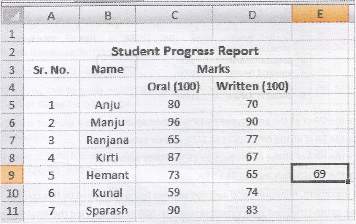
(i) Identify the nature of formula in the cell E9.

(ii) Copy the formula applied in cell E9 to all the cells from E5 to E11.

(iii) Find the maximum and the minimum value among the cells E5 to E11.

(iv) Calculate the average of both Oral and Written marks.

Answer

(i) The formula in E9 is = AVERAGE (C9 : D9). It calculates the average of the marks in cells C9 and D9. It uses the AVERAGE() function.

(ii) When the formula is copied to cells from E5 to E11, the cell references adjust themselves relatively as follows:

E5 = AVERAGE (C5 : D5)

E6 = AVERAGE (C6 : D6)

E7 = AVERAGE (C7 : D7) and so on.

(iii) The maximum value can be calculated by using the formula =MAX(E5:E11). The maximum value is 93.

The minimum value can be calculated by using the formula =MIN(E5:E11). The minimum value is 66.5.

(iv) Ravi can use the formula =AVERAGE(C5:C11) in the cell C12 to calculate the average of Oral marks.

He can use the formula =AVERAGE(D5:D11) in the cell D12 to calculate the average of Written marks.

Question 4

Sahil has been given the hard copy of the following worksheet by his teacher.

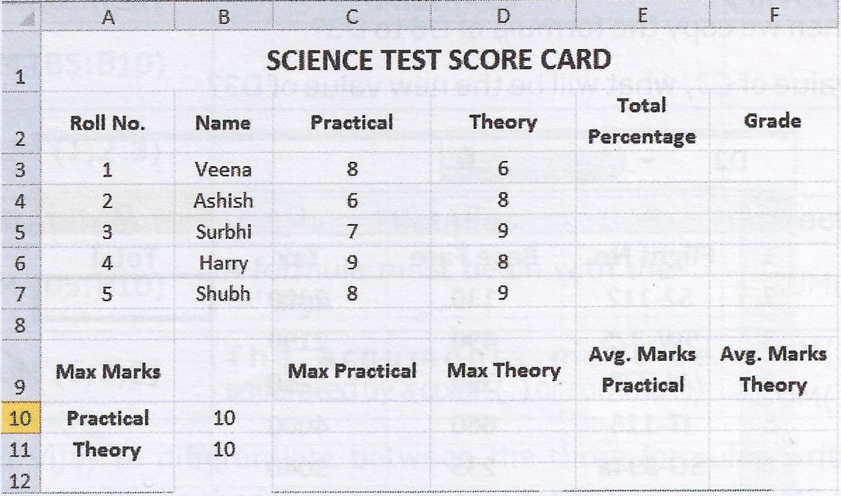
His teacher has asked him to:

(i) Calculate the total percentage of each student.

(ii) Find the Grade of each student by keeping a simple rule in view, i.e., students scoring below 90% must get B+ while those above this baseline must be given an A+.

(iii) Also find the Maximum marks and calculate the average Marks of both Practical and Theory.

Answer

(i) Sahil can calculate the Total Percentage of Veena by using the formula =(C3+D3)/20*100 in cell E3. Then, he can copy the formula in cell range E4 : E7 to calculate the Total Percentage of all students.

(ii) Sahil can calculate the Grade of Veena by using the formula =IF(E3<90, "B+", "A+") in cell F3. Then, he can copy the formula in cell range F4 : F7 to calculate the Grade of all students.

(iii) To find the maximum marks in Practical, Sahil can use the formula =MAX(C3:C7) in cell C10.

To find the maximum marks in Theory, Sahil can use the formula =MAX(D3:D7) in cell D11.

To find the average marks of Practical, he can use the formula =AVERAGE (C3:C7) in cell E10.

To find the average marks of Theory, he can use the formula =AVERAGE (D3:D7) in cell F11.